Archive for the ‘Area’ Category

I’ve had some time on my hands with bus cancellations lately so I decided to fool around with this again (after a 2 year break). Feel free to post comments (both supportive and nasty); I will approve them all.

Integral of cos(x)

Cos(x) integral

Integral of cos(3x)

Cos(3x) integral

Integral of cos(5x)

Cos(5x) integral

Click on Integral of Cos(px) to further explore this procedure and solidify your understanding of this concept as “p” changes.

Thanks for reading.

References

Courant, Richard., John, Fritz (1999). Introduction to Calculus and Analytics: Classics of Mathematics. New York, NY: Springer-Verlag Berlin Heidelberg.

With “Pi day” fast approaching, the timing of this is appropriate. One activity on day one with my introductory calculus students has them throwing toothpicks onto a large sheet of paper containing several strategically spaced parallel lines. After an adequate number of trials, students double that quantity, then divide that result by the number of toothpicks that touched or crossed any line. Once it is determined that the results are always relatively close to π, they want to know why.

This, along with some other discussions and demonstrations, set the stage very nicely for our little journey through introductory calculus. The entry here shows how part of the curiosity initiated on day one will be satisfied.


Buffons’ Needle (setup)

Buffon's Needle


Function Reflects the Moving Needle

Buffon's Needle2


Conclusion

Buffon's Needle4


I’ve included additional notes below to set up the interactive link that follows.

No Hit (wrong combination)

Buffon's Needle3Optional1


Point of Rotation on Line (always intersecting)

Buffon's Needle3Optional

Click on the link provided here to interact with Buffon’s Needle.


Thanks for reading.


Reference: http://mste.illinois.edu/activity/buffon/

Now that the formula for arc length has been determined, we can pursue surface areas of curved solids.

Some students have great difficulty conceptualizing areas on curved surfaces. The problem lies in the fact that they want to use Δx or Δy in the setup, just as they did when calculating volumes of solids and areas over flat surfaces. Since on a curved surface, both x and y are changing in unison; as one changes, so does the other. For this reason, we need to use a variable linking those two variables together. This brings into play the Pythagorean Theorem and arc length. Arc length is a one-dimensional measure, its formula the result of capturing the interplay between Δx and Δy and expressing that as Δs. Integrating the one-dimensional Δs over a given interval will therefore produce the desired outcome (even though the path might not be linear, its distance is nevertheless one-dimensional).

A similar argument can be made for calculating areas over curved surfaces. Since area is two-dimensional, the integral we set up to calculate area must stick to that. I visualize a sphere wrapped with very narrow “bands”. If one of these bands was removed and cut, it could be stretched out and laid flat; its length on one edge would exceed that of the opposing edge due to the fact that it was wrapped around a curved surface. Ultimately this is not a problem, however, since these two opposing edges approach the same length as the distance between them narrows. This is entirely similar to each annulus in a previous post where circle area was derived using the “onion proof“.

This takes care of one dimension required for surface area. The second dimension is arc length mentioned in paragraph two above. As  Δs approaches zero, the line segment joining the two infinitely close points that determine the “point” of tangency becomes ever more perpendicular to the length of each band mentioned earlier. Each band can be treated as a rectangle; area is determined as the product of width (arc length) and length (circumference of 3-D solid) at each x_i over the given interval.


The following notes reveal surface area of a sphere using the reasoning described above.

Sphere

Surface Area (sphere)Conventional

Click on the link to view the changing width of each “band” around the sphere.


As before, students can once again benefit having a second example from which to draw comparisons to the first; the cone serves this purpose very well.

Lateral Surface Area of Cone

Cone Lateral Area


Thanks for reading.

Polar coordinates are not formally introduced in high school, yet sector area is required to prove fundamental trigonometric limits. Having already seen that proof, it wouldn’t be all that painful for students to see circle area derived through the limiting process as applied to angles.

Variable Angle Fixed Radius

Circle AreaPolar


I’ve included another scenario below, this time with variable radius as well.

Variable Angle, Variable Radius


Circle AreaPolar(delta r)

Explore changing polar coordinates here.

Connect your understanding of polar coordinates to that of cylindrical coordinates.


Thanks for reading.

For the past week or so, we’ve been focused primarily on differential calculus and becoming comfortable with the rules that have been derived through the limiting process. The derivatives of e^x and ln(x) were both derived but only the anti-derivative of the former reveals itself through that process. Since the primitive of ln(x) remains a mystery, only the first part of the exploration below can be tackled.

In order to facilitate completion of the entire sequence below, I will ask the students to determine the derivative of f(x)=-x+xln(x). The result will be very useful for our purposes here and will also launch us into Integration by Parts.

AreaUnder exp


AreaUnder exp2


AreaUnder exp3


Thanks for reading.

When working with composite functions, u-substitution often simplifies the integration process for us. What is sometimes overlooked, however, is the significant adjustment that occurs to the area beneath the curve.  The image and link below allow students to explore the significance of this procedure.

ChainRule Area Cos

Interactively explore u-substitution.


As seen below, u-substitution is not a viable approach to integration as its leads to division by zero. In the case below, and others like it, trigonometric substitution provides a means for us to move forward and solve many problems. The process below also brings trigonometric identities into play, thereby  exposing students to their significance.

Circle Area Trig Substitution Formula1

Circle Area Trig Substitution Formula2

Thanks for reading.

As I’ve stated before, circle area would once again be investigated. This iteration brings uniform sub-intervals into play (apologies for all the color but thought it would be helpful for students to distinguish upper and lower bounds).  The link directly below this image opens a new tab from which students can adjust two parameters to explore the partitions; those sliders appear at the right-hand side near the bottom.

Circle Area(2)BLOG

In the image above, there are two rectangles displayed; the length of the blue rectangle is based on the circumference of the upper bound, the length of the red on the lower bound. By reducing the width of each partition (link below), you will see that these two lengths approach a common value.

Interactive exploration of the image directly above.


Circle Proof (Uniform)


For a direct comparison between this version and that using non-uniform partitions, I’ve added the image below.

Fermat Circle

One final note here: Area of the circle using annuli of uniform sub-intervals extends naturally to volumes by cylindrical shells. Walls extend perpendicular to the upper and lower bounds of each annulus; the height of these walls is governed by a function of “x” (single variable calculus). For f(x)=c, the layering effect of cylindrical shells forms a cylindrical solid. For f(x)=ax+c, the solid formed is a cone, if f(x)=ax^2+b, a paraboloid emerges. These are a reasonable conclusions that high school students readily accept. Volumes by slabs follow the same argument. 

Cylindrical Shells

Volume Cone Shells4

I also like to have students set up integrals from both dx & dy perspectives (as seen below).

Paraboloid (shells)


Thanks for reading.

I’ve always liked using the “onion proof” as an easy approach to showing students why the area of a circle is what it is. I also strive to fold in as many previously learned concepts as possible when introducing new ones.  Fermat’s non-uniform partitions provide a very rich approach to deriving areas.  This approach as it applies to the circle is shown directly below.  As you will see, factoring skills that students have learned in Grades 10 and 11 are put to work and out pops the circle’s area; students like this.


The Setup

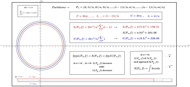
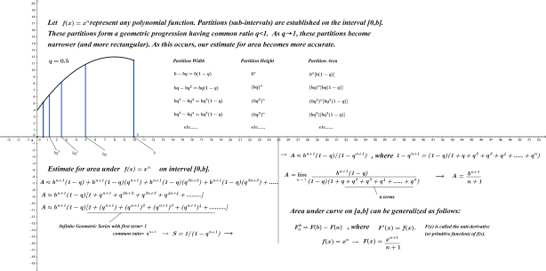
A line on [0,1] was first drawn, then partitions based on q=0.5 identified; those partitions were then summed and the total approached 1 (as it should). This idea was then connected to the formula for sum of infinite geometric series (which was also quickly derived). Additional iterations with q=0.9 and q=0.99 revealed that the non-uniform partitions would become “more uniform” as “q” approached “1”. This idea was then generalized over the interval [0,r] and the lengths of each sub-interval determined.

Concentric circles were eventually drawn around the lower bound of the main interval and the area of each annulus was reasoned out through discussion. It was concluded that the upper bound of each sub-interval could be used to represent the length of each annulus, with the span of the corresponding partition equal to its width. It was agreed upon that these annuli, when”sliced” and “unrolled”, formed rectangles whose areas were easily determined.
Lengths, widths, and ultimately areas of at least 3 of these rectangles were recorded and then summed. Some simple factoring revealed a “new” expression with recognizable components. After some simplification, “q” was replaced with “1” and out popped a very good estimate for the area of a circle.
This process was then repeated for f(x)=x^2 and f(x)=x^3 since the factoring skills required for those was also in place. The entire process was then generalized and applied to the function f(x)=x^n and from this, our expression F(x) was determined.

Shown below are the circle and f(x)=x^n. The links provided here allow students to adjust the common ratios for each and view the resulting partitions.

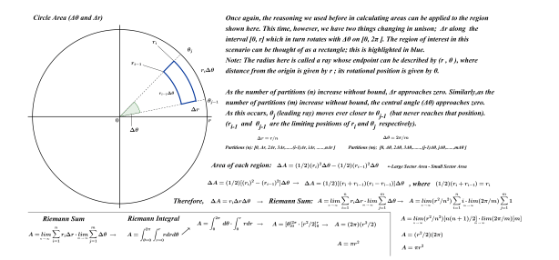
Non-Uniform Partition Exploration: Circle

Fermat Circle

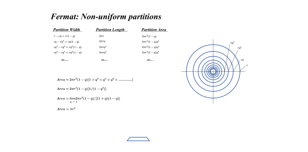
If we were to sketch a function of area “A” with argument “q”, we would find that it has a point of discontinuity at (1,  πr^2). We can say that the function has a limit of  πr^2 as “q” approaches 1.


Non-Uniform Partition Exploration: f(x)=x^n

Fermat

Thanks for looking.


Reference

Courant, Richard., John, Fritz (1999).  Introduction to Calculus and Analytics: Classics of Mathematics. New York, NY:  Springer-Verlag Berlin Heidelberg.

When introducing my high school students to Calculus, I begin by asking them if they would like to see why the volume of a cone is what it is; they invariably respond “yes”.  This leads immediately into some diagrams and discussion on what they already know and information that is missing. I tell them up front that the sum of squares formula will be needed; this is derived through telescopic sums, a rich task in itself.

A diagram of a cone is then sectioned into cylindrical slabs and, through further discussion, it is decided that a reasonable estimate for volume of the entire cone could be determined if these slabs were very thin, there volumes calculated and then summed.  The basic idea behind integration has now been considered and off we go.

By the end of day 2, students have seen how the discrete representation (Riemann sums) gives way to its continuous counterpart (integration) through use of the power rule. We work through several examples with uniform subintervals and then develop the power rule for integration using non-uniform partitions on f(x)=x^n.  The FTC follows shortly thereafter; students are then given some time to practice finding area by setting up simple integrals and working through the process.

Simple differential equations soon follow, as shown below.

Differential Equations.png

Rates of change (and related rates) can very easily be folded into the fabric of our work from thoughtful consideration of the topic shown above.  This is a necessary outcome as the task of deriving integrals of logarithms, trig functions, etc. is too demanding at this level.  Derivatives of these functions are, however, well within the grasp of high school students. Once these are derived, the inverse nature of integrals and derivatives can be exploited to continue on our little journey.

I realize that this approach isn’t for everyone but it works for me and my students seem to enjoy their work as well.

That is all for now. Thanks for reading.