Archive for the ‘Integral Calculus’ Category

I’ve had some time on my hands with bus cancellations lately so I decided to fool around with this again (after a 2 year break). Feel free to post comments (both supportive and nasty); I will approve them all.

Integral of cos(x)

Cos(x) integral

Integral of cos(3x)

Cos(3x) integral

Integral of cos(5x)

Cos(5x) integral

Click on Integral of Cos(px) to further explore this procedure and solidify your understanding of this concept as “p” changes.

Thanks for reading.

References

Courant, Richard., John, Fritz (1999). Introduction to Calculus and Analytics: Classics of Mathematics. New York, NY: Springer-Verlag Berlin Heidelberg.

The power of integral calculus is once again exploited in this entry, this time to determine the centers of mass of one- and two-dimensional objects. Before getting to that, however, some preliminary “discourse” will be engaged in to set the stage.

Everyone (of my age at least) can relate to the scenario involving two children playing on a see-saw. If the children have equal mass and are sitting an equal distance from the fulcrum, they can achieve perfect balance; the fulcrum in this scene is located at the center of mass. If, however, two differing masses are involved (all other things remaining equal), the side containing the greater mass will rotate downward on the fulcrum. This brings us to a very important term for this and other concepts involving rotational motion. This term is called the MOMENT of a force and is defined below:

The moment of a force is a measure of its tendency to rotate about an axis or a point. The moment can be influenced by two quantities: the object’s mass and its distance from the axis or point of rotation; this distance can be referred to as the moment arm.

Moment=Force x Distance , with units measured in ft-lb, kgf-m, etc.

In our example, when two children of the same mass are positioned an equal distance on opposing sides of the fulcrum, a state of equilibrium is achieved. If a bird suddenly joins in the fun and lands on the head of one of the participants, the mass on that end is increased and begins to rotate downward; this increase in mass has created a moment. A moment can also be created if one participant increases his/her position relative to the fulcrum. The moment arm on that side has now been lengthened, thereby creating a moment.


When finding the center of mass in one dimension, the same principles apply; this is a very straight forward procedure if the object has uniform mass density over its entire length. Complications arise, however, if the object’s mass density is not uniform throughout. To address this issue, the object is analyzed as a collection of very small points, each having its own mass and unique position (moment arm) within the main object; each of these will be referred to as “point-mass”.  As in the playground scenario described earlier, the further each point-mass is situated from the axes (or point) of rotation, the greater its contribution will be to the moment and, thereby, its influence on the location of the center of mass. The calculation for center of mass is built upon the concept of weighted averages; while the most frequently occurring outcomes have a significant say with respect to the overall average, the extreme outliers can also have a measurable impact.


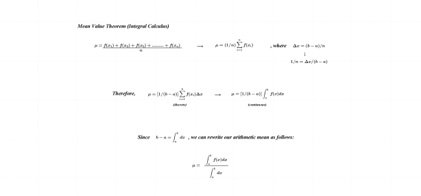
Before weighted averages can be referenced in this context, the notation and the underlying concept that will be utilized throughout must be introduced. This is initiated below in the Mean Value Theorem of integral calculus.

Mean Value Theorem of Integral Calculus

CenterofMassMean Value Theorem

NOTE: In the calculations that follow, x- and y-components of the moment appear. Since centers of mass occur at a point of equilibrium, force due to gravity is ignored and omitted from the units chosen to represent those quantities. I wanted clarification on this item here since moments are once again called upon when dealing with torque. In that application, force is included in the units of measurement when describing moments of inertia.


A reference was made earlier to “point-masses” and their relative position within the object containing them. A direct connection between this and weighted averages exists and is presented below.

Weighted Average

CenterofMassWeighted Average


The end result in the first two examples in the following image are common sense and serve as a “trial run” on the theory developed above; all three can be related directly to our playground scenario described earlier.


One Dimensional Center of Mass

Centers of Mass (examples)


While limiting ourselves here to one-dimension would be silly, attempting to illustrate centers of mass in three dimensions on a 2-D surface could be considered reckless. For this reason, two-dimensions will be the extent to which this topic is pursued here.

Two Dimensions: x-component

Centers of Mass (2D) x-component


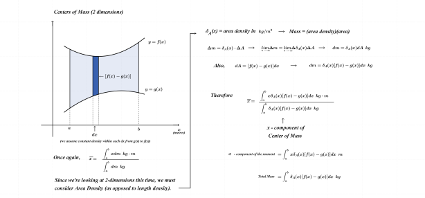
Two Dimensions: y-component

Centers of Mass (2D) y component


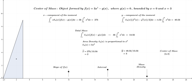
In the examples that follow, centers of mass are determined using the theory developed above. Interactive links also provide the opportunity to change one or more parameters in these examples to observe variations in the various integrals involved.

Constant Function

CenterofMassConstant

Click on the link provided here to interact with centers of mass on one dimension.


Linear Function

Center of Mass example (2D)


One Image from the exploration that follows……

CenterofMassLinear

Click on the link provided here to explore centers of mass defined by linear functions.


Quadratic Function

CenterofMassQuadratic

Click on the link provided here to explore centers of mass defined by quadratic functions.


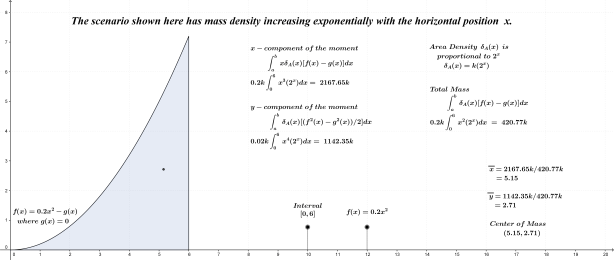
The examples that follow have mass density increasing exponentially along the x-axis. With exponentials in the mix, the need for a new method of integration (by parts) emerges; the power of WolframAlpha is also introduced to do the “heavy lifting”.


Constant Function: Exponential Increase in Mass Density

CenterofMassConstant2a


The x-component of the center of mass in the example above can be calculated manually using integration by parts; this procedure is included here.

Integration by Parts

IntegrationbyPartsCoM


Click on the link provided here to explore centers of mass resulting from an exponential increase in mass density.


While integration by parts can be exploited to evaluate all integrals of this form, the process can become a time-consuming one. The following example is one result obtained from the exploration directly above; it is included here with the intent of introducing students to the power of WolframAlpha. The x-component of the center of mass is shown in a screenshot of the WolframAlpha app available on any device. Interested students have the option of verifying this and other results manually using integration by parts.


Quadratic Function: Exponential Increase in Mass Density 

CenterofMassConstant2


WolframAlpha App

WolframAlpha

I’ve included a link here to the web-based version of the app shown above. To verify the y-component of the center of mass in the final example shown above, click on WolframAlpha.


Thanks for reading.


References

Courant, Richard., John, Fritz (1999).  Introduction to Calculus and Analytics: Classics of Mathematics. New York, NY:  Springer-Verlag Berlin Heidelberg.

Larson, R., Hostetler, R. P., & Edwards, B. H. (1995). Calculus of a Single Variable: Early Transcendental Functions. Lexington, MA: D.C. Heath.

Pressure is a force per unit of area exerted over the surface of an object (as in 35 psi in the tires on your car). When an object is immersed in water, or some other liquid medium, the fluid pressure exerted on that object varies with the depth at which it is submerged. For example, the volume of water pressing down on an object submerged 10 feet is twice that of an object submerged half that depth.

Fluid Pressure (force per unit area) can therefore be defined as follows:

p=wh ,where w = weight density of the fluid h = depth at which the object is submerged

Fluid Force (total force exerted on object) is therefore given by

F=pA ,where A=total area of surface object in question F=whA

According to Pascal’s Law (principle), an object submerged in a fluid is subjected to equal pressure in all directions (at any given depth). For a sheet of metal submerged in water and resting horizontally at a given depth, the fluid force is constant over its entire surface. If, however, the submerged sheet is resting vertically, the entire force exerted over this object by the water varies with depth; the bottom of the sheet will experience more fluid force than its top. In order to determine the total force acting on this vertically oriented sheet, the force exerted on each rectangular cross-section of infinitesimal width (Δy) will be calculated and summed over the object’s entire vertical span; enter integration. With a well-chosen location for the y-axis in our model, the length of each rectangular cross-section can be easily expressed as some variation of f(y).


Rectangular Plate

Fluid ForceRectangularPlate


The example above was relatively simple since f(y) was a constant throughout its vertical span. With shapes whose widths are not constant, the mathematical model can once again vary depending on the perspective chosen. In the examples below, circular plates have been introduced since they provide opportunities for multiple forms of substitution in the integration process, thereby maximizing learning opportunities for students.


The fluid force acting on the ends of a cylindrical water tank is the subject below. I felt that this would be more interesting than imagining the force exerted on a circular plate submerged in a body of water. To simplify matters here, atmospheric pressure and other factors such as sliding forces have been ignored.

Cylindrical Tank: Half-full (Perspective 1)

tank2


Cylindrical Tank: Half-full (Perspective 2)

tank


Cylindrical Tank: Filled to Capacity

tank3


It is worthwhile drawing attention to the forces acting on the ends of top half of the tank filled to capacity (451.34 lb) and the bottom half filled to half capacity (332.8 lb). This type of thoughtful comparison can add to the students’ understanding of this topic.


The two images directly below once again show the two perspectives of fluid forces acting on the ends of our water tank. They are included here to illustrate the contents of the interactive link that follows.

Tank Centered at (0,0)

CircularPlateSubmerged2


Tank Centered at (0,-2)

CircularPlateSubmerged2b

Click on the link provided here to interact with fluid force on the ends of a cylindrical tank.


In the image and link below, the circular end has been removed from the tank and submerged on its own. Once again, various mathematical models could be used to describe this scenario; the one chosen here has placed the origin at the circle’s center.

CircularPlateSubmerged3

Click on the link provided here to interact with fluid force on a submerged vertical plate with center at origin.


The following links will be of interest to some:

Pressure and Buoyancy and Hydrodynamics


Thanks for reading.


Reference
Larson, R., Hostetler, R. P., & Edwards, B. H. (1995). Calculus of a Single Variable: Early Transcendental Functions. Lexington, MA: D.C. Heath.

As mentioned earlier, my students’ first exposure to calculus is from the “Leibniz” perspective. Introducing integration in the first two weeks opens the door to the exploration of many interesting scenarios, including separable differential equations. These lead very nicely to discussions on rates of change,  providing a seamless segue into the land of differential calculus and derivatives.

After students have a firm hold on the concept of differential calculus, I like to shake things up once in a while by throwing in some integration problems. The subject of this entry, shown below, is one such problem. Students are asked to determine the area bounded by the function  f(x)=4/(1+x^2) and the x-axis from  x=0  to  x=1. When the result emerges, students are highly motivated to understand what’s going on. A great discussion ensues and a plan of attack is formulated; this first attempt is a good one but it eventually ends in a stalemate as illustrated below.


Why u-substitution fails

Pi Estimate Natural Log Attempt


Allowing students to travel down the wrong path often leads to greater learning than might otherwise occur; the example above is no exception. Learning various methods of integration is one thing, but knowing when to employ one approach over another is very empowering as well.

The impasse that was reached above provides motivation to seek out another approach; enter trigonometric substitution. This is a very powerful tool in the arsenal once students learn to recognize the circumstances in which it can be used. It is demonstrated below and leads to the conclusion of this problem.


Trigonometric Substitution

Pi Estimate Trig Sub

Other examples of trigonometric substitution can be seen in calculating  circumference  and area of the circle.

Later on this semester, students will be challenged to determined the arc length on the function  f(x)=x^2  over a given interval; trigonometric substitution will once again be deployed. This time, however, the solution will not be determined so easily. The roadblock in this scenario will lead to even greater learning, hyperbolic trig-substitution included.


Thanks for reading.

With “Pi day” fast approaching, the timing of this is appropriate. One activity on day one with my introductory calculus students has them throwing toothpicks onto a large sheet of paper containing several strategically spaced parallel lines. After an adequate number of trials, students double that quantity, then divide that result by the number of toothpicks that touched or crossed any line. Once it is determined that the results are always relatively close to π, they want to know why.

This, along with some other discussions and demonstrations, set the stage very nicely for our little journey through introductory calculus. The entry here shows how part of the curiosity initiated on day one will be satisfied.


Buffons’ Needle (setup)

Buffon's Needle


Function Reflects the Moving Needle

Buffon's Needle2


Conclusion

Buffon's Needle4


I’ve included additional notes below to set up the interactive link that follows.

No Hit (wrong combination)

Buffon's Needle3Optional1


Point of Rotation on Line (always intersecting)

Buffon's Needle3Optional

Click on the link provided here to interact with Buffon’s Needle.


Thanks for reading.


Reference: http://mste.illinois.edu/activity/buffon/

I’ve never liked the idea of handing students formulas to use without any knowledge of where they originate. Integrals are no different; I believe its easier for students to grasp the idea of integration by setting up Riemann sums first. From this perspective, students can focus on just one “member” in the group of infinitely numerous elements and, from that perspective, build representations for area, volume, force, work, etc. Once students have an expression for that single member, the more abstract integral can be more easily conceptualized.

The entry below describes multiple components working in unison to determine the work required to lift water up and over the edge of a container. The applet provided allows students to interact with two variables (depth & lower radius) and observe how changes to those influence the corresponding algebraic representations. This scenario of lifting columns of water is directly related to the work required to raise a length of chain upwards by a given distance; an example of this follows as well.


Cylindrical Container

VariableWork1


Conical Container

VariableWork2


Click on the link provided here to explore a variable column of water.


I’ve added the following scenario for additional contrast/comparison. This example illustrates rectangular slabs of water being lifted over the upper edge of a v-shaped trough.

V-Shaped Trough

V-Trough3Work

Click on the link provided here to better visualize work required to remove rectangular slabs from a container.


Lifting a Chain

ChainWork


Click on the link provided here to lift a chain.


Work as a Function of Distance (y)

Work over Distance


Click on the link provided here to explore dW/dy.


I wanted work described in terms of “ft•lb” here since students have been exposed to that terminology with respect to torque (rotational analog of work). A later entry will be focused on this which will, in turn, open the door to an exploration into horsepower.


Thanks for reading.

As in the case of the cone, volume of the pyramid can be determined in various ways. The version here once again dabbles with a multi-variable scenario to give students some variation on a familiar theme.

Pyramid Volume2

Click on the link to interact with the notion of infinitesimals as applied to pyramid volume.

Refer to volume of cone for helpful comparison.


Thanks for reading.

Now that the formula for arc length has been determined, we can pursue surface areas of curved solids.

Some students have great difficulty conceptualizing areas on curved surfaces. The problem lies in the fact that they want to use Δx or Δy in the setup, just as they did when calculating volumes of solids and areas over flat surfaces. Since on a curved surface, both x and y are changing in unison; as one changes, so does the other. For this reason, we need to use a variable linking those two variables together. This brings into play the Pythagorean Theorem and arc length. Arc length is a one-dimensional measure, its formula the result of capturing the interplay between Δx and Δy and expressing that as Δs. Integrating the one-dimensional Δs over a given interval will therefore produce the desired outcome (even though the path might not be linear, its distance is nevertheless one-dimensional).

A similar argument can be made for calculating areas over curved surfaces. Since area is two-dimensional, the integral we set up to calculate area must stick to that. I visualize a sphere wrapped with very narrow “bands”. If one of these bands was removed and cut, it could be stretched out and laid flat; its length on one edge would exceed that of the opposing edge due to the fact that it was wrapped around a curved surface. Ultimately this is not a problem, however, since these two opposing edges approach the same length as the distance between them narrows. This is entirely similar to each annulus in a previous post where circle area was derived using the “onion proof“.

This takes care of one dimension required for surface area. The second dimension is arc length mentioned in paragraph two above. As  Δs approaches zero, the line segment joining the two infinitely close points that determine the “point” of tangency becomes ever more perpendicular to the length of each band mentioned earlier. Each band can be treated as a rectangle; area is determined as the product of width (arc length) and length (circumference of 3-D solid) at each x_i over the given interval.


The following notes reveal surface area of a sphere using the reasoning described above.

Sphere

Surface Area (sphere)Conventional

Click on the link to view the changing width of each “band” around the sphere.


As before, students can once again benefit having a second example from which to draw comparisons to the first; the cone serves this purpose very well.

Lateral Surface Area of Cone

Cone Lateral Area


Thanks for reading.

Surface areas of curved 3-dimensional solids tend to be much more difficult for students to conceptualize than those whose sides do not stray from a “level” plane. These will eventually be addressed but we will first discover how to calculate lengths of curves.

The circle will once again be called upon to initiate this exploration; the image below illustrates, in part, the method of exhaustion that Archimedes utilized to arrive at his estimate for π.

Archimedes Circumference2

Click on the link here to interact with what Archimedes revealed.


……..and now this. Was Archimedes wrong???

IMG_5215

Source: math.stackexchange.com

If the fellow above had joined pairs of points at each successive corner with a line segment (hypotenuse) and based his calculation for circumference on the sum of those, he would have found that Archimedes was correct all along.


Arc Length Formula

As  Δs approaches zero in this exploration, its length becomes a more accurate estimate for the arc length near the “point” of tangency (there are always two points in very close proximity). The end result through the limiting process shown directly below is the formula for arc length.

ArcLength Circle

Its always beneficial for students to work through several examples to cement their understanding of new concepts and related procedures; my preference is to provide examples that are already familiar to them. Calculating arc length (in this case) can then serve as a verification and acceptance of the new concept is achieved with confidence. The offering directly below and the link that follows connects the arc length formula to the Pythagorean theorem.

Arc Length

The formula for arc length is based on the Pythagorean theorem; it is therefore not surprising that they produce the same lengths on linear functions.


The real power of the formula for arc length lies in its applications to curves. Since students have known the circle’s circumference for several years, it is appropriate to now derive 2πr using our new tool. This is shown below and once again brings trigonometric substitution into play.

Circumference of the Circle

Arc Length (Circumference of Circle)

Once the circle’s circumference has been established using the arc length formula, the integration process can be further solidified by using arc length to once again calculate the circle’s area.


The formula for arc length will once again be employed in deriving the formulas for surface area of the sphere and cone.


Thanks for reading.


This entry will no doubt get further under the skin of those who contend that I’m pushing things too far (and that is exactly why I’m publishing it).  This is a natural extension of the 2-dimensional analog in which circle area was derived. Cylindrical coordinates are identical to polar coordinates with a 3rd dimension thrown in. Directly below, the vertical dimension is governed by a linear function which results in a cone.

In the spirit of consistency, I’ve included a second example with which to draw comparisons to the first. Everything is identical between the two cases with one exception; the function which governs the vertical dimension in example two is that of a semi-circle.


Volume of a Cone

VolumeCone Cylindrical

Interact with cylindrical coordinates to see how the 3-dimensional sector changes.


Volume of a Sphere

VolumeSphere Cylindrical


Thanks for reading.