First Week
Day 1
The branch of mathematics called “calculus” was defined as the “mathematics of change”. A discussion of the movement of a point residing on the Earth’s equator and the corresponding position function was determined. Slopes of this function at the critical points were determined, interpreted and compared to a second function (derivative of the displacement function). With the help of technology to determine slopes, connections quickly became apparent between rates of change of the displacement function with respect to time and the value of the second function. Students immediately wanted to know more and were informed that they would soon learn an efficient method of determining rates of change.
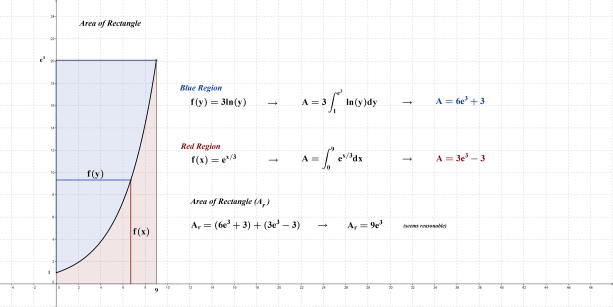
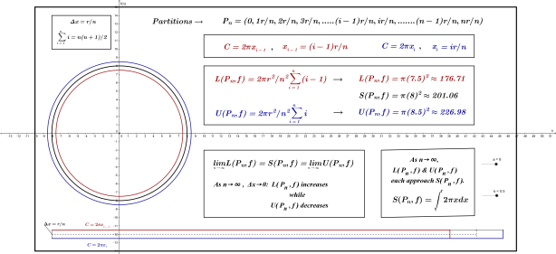
Buffon’s experiment was also recreated and an estimate for π emerged. I mentioned to students that the reasoning behind this method will be constructed by the middle of March (π week). Students were also informed that probability and calculation of areas would be required to meet this challenge.
The two branches of calculus had now been introduced within the first 40 minutes of our 80 minute block. Following a very brief discussion of what Newton and Leibniz contributed to mathematics, the students were primed to further investigate either branch.
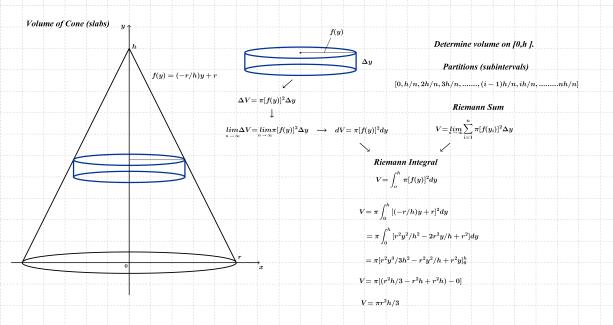
It was decided that we would spend the remainder of our class time investigating the volume of a cone. The formula for sum of triangular numbers was quickly determined; this was followed by a more lengthy derivation of the formula for sums of squares (using telescoping sums). With these in place, a linear function having slope r/h was drawn through the origin. I asked the students to imagine what shape would emerge if we could rotate that line around the x-axis; a cone was visualized and notion of volumes of revolution introduced. I quickly sketched a cross-sectional slab of thickness ∆x; this cylindrical slab was duplicated away from the cone and its volume was quickly identified. Discussion ensued with respect to similar cross-sectional slabs cut from other positions on the cone; students immediately noticed that the radius varied and was governed by the linear function f(x)=(r/h)x.
Students quickly agreed that by calculating volumes of individual slabs and summing (integrating) those on the interval [0, h], a reasonable estimate for the cone’s volume should emerge. Uniform sub-intervals of length ∆x=(h/n) were then established and recorded on the white board. Students accepted the idea that if “n” were to increase without bound, the cylindrical slabs would become increasingly narrow and the estimate for the cone’s volume would become more precise.
It was then decided that the radius of each slab “f(x)” could be based on the upper bound of each sub-interval (since all values of ” x ” from there to the lower bound become infinitely close to one-another as “n” increases without bound). Following some factoring, an appropriate substitution of the sum of squares formula and evaluation of limits as “n” moves to an infinitely large value, the well-known formula for volume of the cone appeared; minds blown (in a good way).
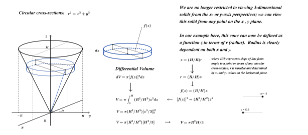
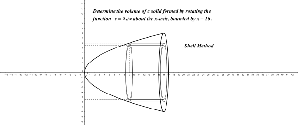
We will soon turn the cone onto its base and calculate volume by horizontal slabs (as shown directly below) and eventually by cylindrical shells (lower image).
Horizontal Slabs
Cylindrical Shells

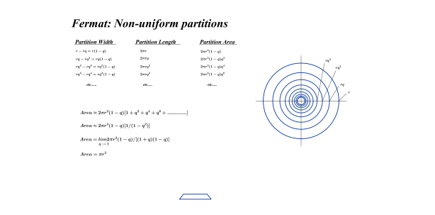
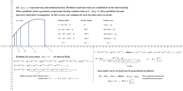
Later in the week, the power rule for integral calculus was derived using Fermat’s non-uniform sub-intervals as shown in the image below; the Fundamental Theorem of Calculus was also established at this point. The cone’s volume was once again derived by adding volumes of slabs sliced from uniform sub-intervals. Students now discovered that these discrete volumes (Riemann sums) gave way to their continuous counterpart (Integral). Applying the power rule of integration to π((r/h) x)^2 and evaluating the result over the interval [0, h] using the FTC quickly produced the desired formula. The integral notation was adopted soon thereafter.
Fermat’s Non-Uniform Partitions
The time remaining over the final two days of Week 1 primarily involved students setting up and evaluating integrals; primitives of functions for which the power rule did not work were provided as the assignment given included those as well. The primitives of these functions will later be determined and defined further as anti-derivatives through the use of differential calculus.
Second Week
Day 1
A review of the previous week’s topic was followed by the introduction of rates of change. The introduction of a new topic always involves discussion and students are asked to avoid note-taking; engagement in discussion, diagrams and analysis is maximized in this way. What is learned on day 1 will be summarized with carefully scripted notes the following day (discussion is always included here as well for clarification when needed).
The function f(x)=x^2 was used initially with a secant line drawn between two distinct points P and Q. An expression for the slope of this line (average rate of change) was determined for “x” and “(x+∆x)”. A right triangle was then sketched and the slope of the line segment PQ was related to the tangent ratio of the angle formed at point P. It was then determined that the tangent line at P would become the limiting case of secant PQ (since ∆x can never be zero). A direct comparison to points of discontinuity from Math 30 was also made here. We will discuss left- and right-hand limits to determine whether or not a function is differentiable at a given point later on this semester; it is an unnecessary distraction at this point.
Preceding the delivery of my notes on day 2, the drill from the previous day was repeated, this time with f(x)=x^3. When comparing the results from the two functions, a pattern seemed to have emerged. Having seen this limiting process twice, the notes on differential calculus would now have some meaning to students. The term “derivative” was introduced and shown that it is itself a function. Various notations of the derivative were also introduced here (Leibniz, Lagrange, Newton) as were numerical representations. Several examples of f'(x) and f'(a) were worked through in class together and then time given for students to practice.
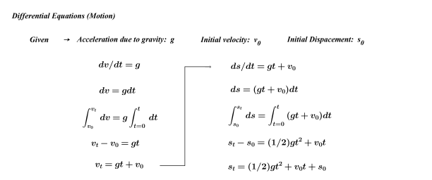
When students need a break from practice, I give them something new to think about. On day 3, we brought some simple physics into play. Students already know that acceleration is the rate of change of velocity with respect to time; dv/dt=a. Since they learned simple differential equations in week one, the equation above was re-written as dv=(a)dt.
The following exchange ensued:
Question: What can we do when “dv=(a)dt” shows up in this way?
Answer: We can integrate.
Question: What does integration give us?
Answer: The area between the function and the x-axis.
Question: What does our function represent?
Answer: Acceleration.
Question: What does the area in question represent?
Answer: Velocity.
Question: Have you ever seen this before and, if so, where?
Answer: Yes, in Physics class.
Comment: Now you know why Newton invented calculus!
Getting back to our differential equation…….
The process of integration above resulted in v=at+v_0.
We then executed the same process once again, this time for ds/dt=v.
Repeat question/answer sequence.
Through the integration of ds=(at+v_0)dt, the displacement function encountered so many times in Math 20-1 (and Physics 20) appeared.
s=(a/2) t^2+(v_0) t+s_0
This happens very quickly and gets students thinking. It also brings back the topic of integration and sets up very nicely the inverse relationship between derivatives and integrals.
Other “extras” that were thrown in during week 2:
-Chain Rule using Leibniz notation and “u”substitution.
-proof of fundamental trig limits
-derivative of sin(x) through algebraic analysis and graphing
Additional information given but not yet derived:
-product rule: d(fg)=f’g+g’f
-quotient rule: d(f/g)=(f’g-g’f))/g^2
– d/dx ln(x)=1/x
– d /dx cos(x)=-sin(x)……this was reasoned out using graphs.
Upcoming:
-derivatives of ln(x),e^x,cos(x) and proofs of product & quotient rules using logarithms.
-setting up and solving simple differential equations from slope fields
-further analysis of significance of chain rule as it applies to derivatives AND integrals. This analysis will occur both geometrically and analytically.
-linear regression using method of least squares.
By the end of February, students will be quite fluent in setting up and solving simple problems involving derivatives and basic integrals. Further work with limits and curve sketching will be done later in the semester and will seem trivial by that time.
It is clear from this entry that I am a “constructivist”. I realize that some proponents of discovery learning will hammer on me for this; that is fine. There is still plenty of room in this approach for students to explore and discover connections on their own. Differentiation and integration are tools for other pursuits, not an end in themselves. This not meant to insult high school math students but it would take them much longer than 2 weeks to be in the position we presently find ourselves.
Between now and the end of this semester, we will continue to explore circle area, cone volume, arc length, etc. and through those pursuits, trigonometric substitution, integration by parts and partial fractions will eventually emerge; the proof of Buffon’s needle experiment in the middle of March will seem anti-climactic. Logistic growth, work, centers of mass in 1- & 2-dimensions, and other more complex applications of calculus will also be pursued and tackled.
That’s all I have to say for now.
Thanks for reading.
Reference: Courant, Richard., John, Fritz (1999). Introduction to Calculus and Analytics: Classics of Mathematics. New York, NY: Springer-Verlag Berlin Heidelberg.
55.152185
-118.814114