Archive for the ‘The Derivative’ Category

The main subject of this entry was originally planned as an optimization problem involving differential calculus only; its been slightly modified. This more interesting approach provides the derivative up front, presenting students with three separate tasks to pursue from that point. As a consequence, students are reintroduced to differential equations and curve sketching.

A talking point emerges as well: Is there a difference between derivatives and differential equations?


Inscribed Triangle of Maximum Area

Inscribed Triangle animation


Click on the link provided here to explore area of the inscribed triangle.


Thanks for looking.

By the time curve sketching is formally introduced, students have already seen a few “purposeful” examples; they are listed below as links.

Putnam Problem, Four Townse^(Pi) vs (Pi)^ef(x)=x^x (L’Hospital’s Rule)

Through these examples (and others), first and second derivatives have been points of discussion with respect to identifying the location and nature of critical points. In addition to this, L’Hospital’s Rule will have been established along the way and thrown into the mix.

My formal introduction to curve sketching is introduced in the form of a problem solving scenario. An example of this is shown below.


Sum of a Number and its Reciprocal

Curve Sketching


Limits at Infinity & Infinite Limits

Curve Sketching2


First and Second Derivatives

Curve Sketching3


Graph of   S(x) = x + 1/x

x + 1 by x

Click on the link provided to interactively determine the local extrema.


Graph of   y=sin^2(2x)/x^2  (see L’Hospital’s Rule for indeterminate limits of this function)

L Hospital's Rule Second Iteration2

Click on the link provided here to explore the relationships between  y, y’ and y”.


Thanks for reading.

In the spirit of consistency, several additional examples supplementing my introduction to related rates are included here. As seen in the first example below, past concepts are revisited and, in turn, connected to newly introduced ones. Mixing things up from that point on provides students with a variety of perspectives on the same theme that serves to further cement understanding.


Separable Differential Equation

Circle area Derivative


Three Approaches to Related Rates

Circle area Differential Equation


Application to Conical Container

DiffEqua Realted Rates2


Rate of Change of Arc Length

DiffEquaRelatedRatesArcLength


The approach to solving each of these related rate problems is the same; identify what is known, what is desired and then connect the two.


Thanks for reading.

Now that the formula for arc length has been determined, we can pursue surface areas of curved solids.

Some students have great difficulty conceptualizing areas on curved surfaces. The problem lies in the fact that they want to use Δx or Δy in the setup, just as they did when calculating volumes of solids and areas over flat surfaces. Since on a curved surface, both x and y are changing in unison; as one changes, so does the other. For this reason, we need to use a variable linking those two variables together. This brings into play the Pythagorean Theorem and arc length. Arc length is a one-dimensional measure, its formula the result of capturing the interplay between Δx and Δy and expressing that as Δs. Integrating the one-dimensional Δs over a given interval will therefore produce the desired outcome (even though the path might not be linear, its distance is nevertheless one-dimensional).

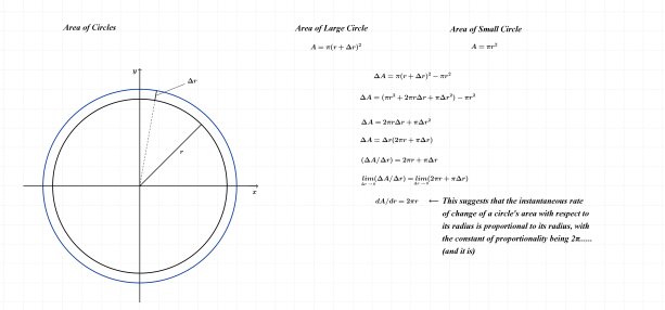
A similar argument can be made for calculating areas over curved surfaces. Since area is two-dimensional, the integral we set up to calculate area must stick to that. I visualize a sphere wrapped with very narrow “bands”. If one of these bands was removed and cut, it could be stretched out and laid flat; its length on one edge would exceed that of the opposing edge due to the fact that it was wrapped around a curved surface. Ultimately this is not a problem, however, since these two opposing edges approach the same length as the distance between them narrows. This is entirely similar to each annulus in a previous post where circle area was derived using the “onion proof“.

This takes care of one dimension required for surface area. The second dimension is arc length mentioned in paragraph two above. As  Δs approaches zero, the line segment joining the two infinitely close points that determine the “point” of tangency becomes ever more perpendicular to the length of each band mentioned earlier. Each band can be treated as a rectangle; area is determined as the product of width (arc length) and length (circumference of 3-D solid) at each x_i over the given interval.


The following notes reveal surface area of a sphere using the reasoning described above.

Sphere

Surface Area (sphere)Conventional

Click on the link to view the changing width of each “band” around the sphere.


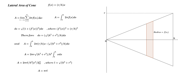
As before, students can once again benefit having a second example from which to draw comparisons to the first; the cone serves this purpose very well.

Lateral Surface Area of Cone

Cone Lateral Area


Thanks for reading.

For the past week or so, we’ve been focused primarily on differential calculus and becoming comfortable with the rules that have been derived through the limiting process. The derivatives of e^x and ln(x) were both derived but only the anti-derivative of the former reveals itself through that process. Since the primitive of ln(x) remains a mystery, only the first part of the exploration below can be tackled.

In order to facilitate completion of the entire sequence below, I will ask the students to determine the derivative of f(x)=-x+xln(x). The result will be very useful for our purposes here and will also launch us into Integration by Parts.

AreaUnder exp


AreaUnder exp2


AreaUnder exp3


Thanks for reading.

Having previously determined the derivative of ln(x), we now have that at our disposal to show one perspective of the product and quotient rules of differential calculus. A quick excursion to “implicit differentiation land” and a review of the chain rule will set things up nicely to meet our objectives here.

Implicit Diff and Chain Rule


Product and Quotient Rules

Product Quotient Rules

Modified Product Rule

Modified Product Rule

Thanks for reading.

Once students have a feel for calculating derivatives by limits of various functions, the same is done for ln(x) and e^x. Each of these show the importance of binomial expansion as that skill is once again necessary in understanding why things are as they are.

Derivative of ln(x)

Derivative(ln)

The derivative of ln(x) have many applications including logistic growth which we will see later this semester. We can, however, put this to work immediately by using it along with our knowledge of the product and quotient laws of logarithms. These are woven together nicely to determine the product and quotient rules of differential calculus.

The Euler constant “e” is also exploited in deriving the Rule of 72.


Derivative of e^x

Derivative(e^x)


Geometric Perspective of d(a^x)/dx

Derivative Exponential Function

To interact with the function above, click on d(a^x)dx.

Click the link provided to see two additional perspectives on the derivative of e^x.


Thanks for reading.


Reference

Courant, Richard., John, Fritz (1999).  Introduction to Calculus and Analytics: Classics of Mathematics. New York, NY:  Springer-Verlag Berlin Heidelberg.

Yes, I prefer introducing integral calculus prior to differential for various reasons, one of which is that I believe that the former should not be dependent on the latter (my reasoning for this approach is very sound, in my opinion). The two disciplines are each introduced on their own merits with the inverse relationship between the two being discovered soon thereafter. These are my notes introducing differential calculus.

Derivative

Derivative2Derivative3


Click on secant line and adjust slider.

Thanks for looking.


Reference

Courant, Richard., John, Fritz (1999).  Introduction to Calculus and Analytics: Classics of Mathematics. New York, NY:  Springer-Verlag Berlin Heidelberg.

When introducing my high school students to Calculus, I begin by asking them if they would like to see why the volume of a cone is what it is; they invariably respond “yes”.  This leads immediately into some diagrams and discussion on what they already know and information that is missing. I tell them up front that the sum of squares formula will be needed; this is derived through telescopic sums, a rich task in itself.

A diagram of a cone is then sectioned into cylindrical slabs and, through further discussion, it is decided that a reasonable estimate for volume of the entire cone could be determined if these slabs were very thin, there volumes calculated and then summed.  The basic idea behind integration has now been considered and off we go.

By the end of day 2, students have seen how the discrete representation (Riemann sums) gives way to its continuous counterpart (integration) through use of the power rule. We work through several examples with uniform subintervals and then develop the power rule for integration using non-uniform partitions on f(x)=x^n.  The FTC follows shortly thereafter; students are then given some time to practice finding area by setting up simple integrals and working through the process.

Simple differential equations soon follow, as shown below.

Differential Equations.png

Rates of change (and related rates) can very easily be folded into the fabric of our work from thoughtful consideration of the topic shown above.  This is a necessary outcome as the task of deriving integrals of logarithms, trig functions, etc. is too demanding at this level.  Derivatives of these functions are, however, well within the grasp of high school students. Once these are derived, the inverse nature of integrals and derivatives can be exploited to continue on our little journey.

I realize that this approach isn’t for everyone but it works for me and my students seem to enjoy their work as well.

That is all for now. Thanks for reading.


Four towns (A, B, C, D) are situated to form a square with side length of 1 unit. Determine the minimum length of roadway that will link these four towns together.

View the James Grime video first.

Minimum Length

Click on the following link for an interactive exploration: GeoGebra


The graph below shows the length of roadways linking these towns as a function.

Length as a Function of  “x”

Four Towns Minimum

Click on the link provided here to determine local minimum.


Thanks for reading.