The following is a geometric interpretation of the product rule which is then used to in determining the quotient rule.

Product Rule

If you would like to waste a minute or two, feel free to click on this link to change “h”. For another perspective on the product and quotient rules, click here.

I usually use trigonometric functions to get at this concept but have not yet gotten to those; this worked quite well. Click on the links at the bottom to explore further.

ChainRule Integral


Click here for variations of (ax)^.5.  For a similar experience, click on integrating cosine.

Integrating x^2

Posted: March 1, 2018 in Calculus: An Introduction


Integral x^2

Click on f(x)=(px)^2 to explore variations of the integral above. It would be much more direct to rewrite and integrate as f(x)=p^2(x^2) but that option is not available for many functions. For that reason, I opted to show the process unfold with “p” affecting the function horizontally.  This same process is seen in the Riemann Integral of Cos(px)

I’ve had some time on my hands with bus cancellations lately so I decided to fool around with this again (after a 2 year break). Feel free to post comments (both supportive and nasty); I will approve them all.

Integral of cos(x)

Cos(x) integral

Integral of cos(3x)

Cos(3x) integral

Integral of cos(5x)

Cos(5x) integral

Click on Integral of Cos(px) to further explore this procedure and solidify your understanding of this concept as “p” changes.

Thanks for reading.

References

Courant, Richard., John, Fritz (1999). Introduction to Calculus and Analytics: Classics of Mathematics. New York, NY: Springer-Verlag Berlin Heidelberg.

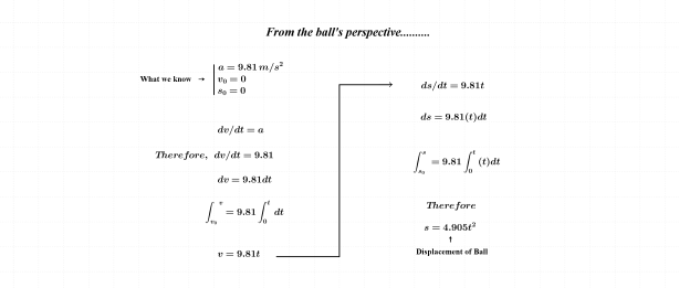
As noted above, the subject of this entry is first order differential equations. Before getting directly to that, however, a few examples of more basic equations representing rates of change will be reflected on.

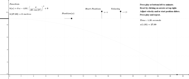
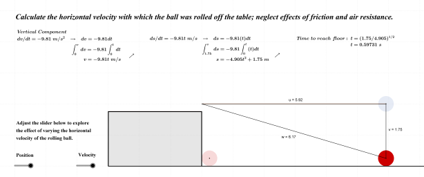
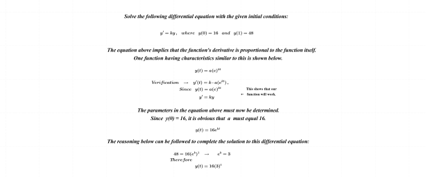
Too often, students are given rules and algorithms to follow in “solving” problems. While becoming fluent with these procedures is not unimportant, students relying on these strategies alone will eventually find themselves swimming in a pool of confusion when faced with unfamiliar looking problems; if problems not recognizable, they become impossible to resolve. In an effort to minimize such predicaments, an intuitive perspective can often be helpful. Directly below are two examples of solutions to basic differential equations; the first resulting in a quadratic function, the second being exponential. The first two frames below show an “intuitive” approach to solving these problems while the third frame shows a more typical procedure.

Quadratic Function

Separable Diff EquationsA2

Exponential Function

Separable Diff EquationsB

Procedure using Leibniz Notation

Separable Diff EquationsA

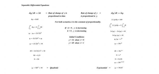
An intuitive feel is supplementary to the procedures shown above and can add understanding to the process. Equally important is developing the ability to create these mathematical models from information conveyed in the written word.

A huge stumbling block for many students is knowing why a specific model works for one scenario and not the next; the deciding factor is sometimes a seemingly small detail that is easily overlooked early in the learning process. The example below draws attention to this and will serve as a bridge between simple separable differential equations and the more complex first order linear differential equations.

Mixing Problems and Solution Concentrations

This portion of our journey will focus on the changing concentration of a solution in a container as the ratio of solute to solvent increases or decreases. One such example is provided below.

A tank initially contains 50 gallons of brine in which 5 lb of salt is dissolved. Brine containing 1 lb of salt per gallon flows into the tank at a constant rate of 4 gal/min. The concentration of the brine in the tank is kept uniform throughout the tank by stirring. While the brine is entering the tank, brine from the tank is also being drawn off at a rate of 2 gal/min. Find the amount of salt in the tank after 25 minutes.

(Fraleigh, p.903)

In this scenario, the concentration of brine being added to the tank differs from that originally present with the new mixture being drained off simultaneously; this is the “small detail” making the problem here a more complex one than the other examples cited earlier. The two frames immediately below illustrate simplified versions of this and will serve as an introduction to mixing problems; both allow for a straight forward model involving separable differential equations.

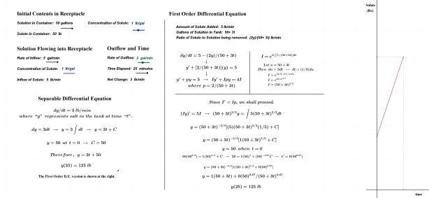
In the scenario directly below, the concentration of solute initially contained in the tank has been altered to match that which is being added (1 lb/gal). That being the case, the concentration of solution being drained away will be a constant 1 lb/gal as well; the resulting function will therefore be linear.

Separable Differential Equation (Equal Concentration)

DiffEquSolution(Constant)1.EqualConcentration1

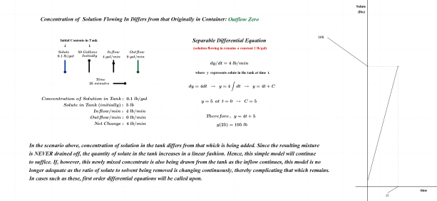
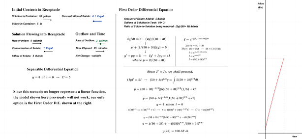
This second example sees the concentration initially contained in the tank revert to 0.1 lb/gal with inflow of 1 lb/gal. This time, however, no solution will be drawn from the container, once again resulting in a linear function.

Separable Differential Equation (Outflow Zero)

DiffEquSolutionOutflowZero1

First Order Differential Equations

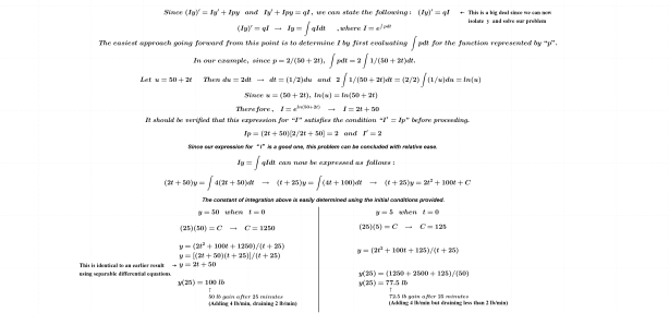
It is now time to tackle the problem posed by Fraleigh. To reiterate, the concentration of solution flowing into the container differs from that initially present AND this new mixture is being drawn off simultaneously, thereby requiring a more complex model. Since the concentration of solution being extracted is constantly changing, that quantity will be expressed as a ratio of salt (in lbs) to number of gallons of brine in the container at any time “t”. Since the quantity of salt in the tank is changing continuously, a variable will be assigned to represent that quantity; we’ll use  “y” to denote pounds of salt.

                                   Inflow:  4 gal/min  at  1 lb/gal  →  4 lb/min                                                                                            Outflow:  2 gal/min  at  y lb/(50+2t) gal  →  [2/(50+2t)]y lb/min

From this, we can easily represent the rate of change of salt (in lbs) with respect to time as follows:

                                                      dy/dt=4-[2/(50+2t)]y    (lb/min)

This expression is referred to as “Item 2” in the frame directly below. The “item” preceding that is a reminder of the FTC that is called upon in solving for what is referred to as an “Integrating Factor”. Its purpose is also discovered below and is denoted by “I”.

Integrating Factor

DiffEquationsImportantNotes.1

Purpose of the Integrating Factor (clarification)

Given    Iy’+Ipy=qI  

If     (Iy)’=Iy’+Ipy , then     (Iy)’=qI     which leads to     Iy=∫qIdt            

The integrating factor ultimately allows us to express  “y” as a function of  “t” (which is our objective).

While first order differential equations are not required in cases where the concentration of inflow equals that already in the container, initial conditions for that scenario are nevertheless included below. The solution to Fraleigh’s problem is shown as well (bottom right) for comparison purposes.

Solution to Fraleigh’s Problem

DiffEquationsImportantNotes.2

To reiterate: If the concentration of solution flowing into the container is equal to that already present OR outflow is zero, the function describing quantity of solute will be linear in nature. The following three frames serves as examples of this important detail.

Linear Function: Constant Concentration (1 lb/gal)

DiffEquationsImportantNotes.4

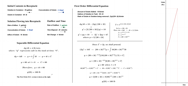
Linear Function: Constant Concentration (2 lb/gal)

DiffEquSolution(Constant)2EqualConcentration

Linear Function: Zero Outflow

DiffEquSolution(Constant)2OutflowZero

The frame that follows is a variation of the problem posed by Fraleigh, this time with an inflow of 5 gal/min. A graph of the resulting non-linear function is also included.

Non-Linear Function

DiffEquationsImportantNotes.5

For further comparison and analysis, I’ve included two additional scenarios directly below, each with an interactive link.

Inflow Exceeds Outflow

DiffEquSolution(Constant)2Alternate2.IntflowGreaterThanOutflow

Click on the link provided here to explore scenarios where inflow exceeds outflow.

Outflow Exceeds Inflow

DiffEquSolution(Constant)2Alternate2.OuttflowGreaterThanInflow

Click on the link provided here to explore scenarios where outflow exceeds inflow.

The following image illustrates the function shown directly above on a different scale. The lack of symmetry here creates additional opportunities for discussion with respect to the rate at which the quantity of solute is changing over time. For example, at t=11.16 minutes it can be stated that the quantity of solute flowing in equals that which is flowing out. What is happening before and after that point in time and why? Is this a reasonable conclusion and does the graph of our function reflect that?

DiffEquDerivativeCheckDiffEquation

Nearly the end………….

I had initially planned on ending this entry with the previous frame; my students, however, wanted one more day to explore mixing problems. I’ve decided to summarize that final day’s sequence here.

As always, this mixing problem began as follows:

                                 y’=q-py  , where   y’ = rate of change of solute (lb/min)                                                                                                        q  = inflow of solute (lb/min)                                                                                                                      py = outflow of solute (lb/min)

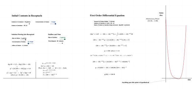
We then decided initial conditions, concentration of solute being added as well as rates of inflow and outflow. The first set of values chosen produced what we thought was a reasonable solution until that function’s stationary point was determined; it occurred at (31.53,-1.96). These values caused some concern so our work was double checked. Since the math seemed to be fine, we decided to graph our function and interpret that. Once everything was taken into consideration, this result was perfectly logical. The tank initially contained 150 lbs of solute (3 lbs/gal); we were adding only 0.2 lb/gal at a rate of 6 gal/min and draining away the diluted mixture at a rate of 8 gal/min. Upon reflection, our result seemed perfectly reasonable. This scenario and resulting function are shown immediately below.

Rapid Dilution

DiffEquSolution(Constant)2Alternate2.BrineOutflowlargerthanInflowAnimation.TrialRun.1

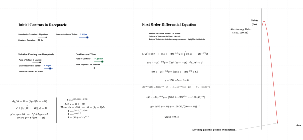
Following our satisfactory explanation of the dilution scenario above, the discussion focused on what would need to change so that the function would produce a maximum value greater that 150 lb (the initial content). It was decided that increasing the concentration of solute flowing in would produce the desired result. A concentration of 4 lb/gal was agreed upon and the function reworked. Upon graphing this new function, the location of its maximum was revealed. The question immediately asked was ‘Why is the maximum located at t=0?’. The derivative was determined and set equal to zero, quickly satisfying everyone. The frame immediately below illustrates this scenario.

Local Maximum at t=0

DiffEquSolution(Constant)2Alternate2.BrineOutflowlargerthanInflowAnimation.TrialRun.2

To further solidify our understanding of this concept, it was decided that the vertex of our graph should move to the right if the concentration of solute flowing in was further increased. This final iteration of our mixing problem is shown in the following frame.

Local Maximum at t>0

DiffEquSolution(Constant)2Alternate2.BrineOutflowlargerthanInflowAnimation.TrialRun.3

Click on the link provided here to further explore mixing problems.

The end.

Thanks for reading.

References

Kline, Morris. (1998). Calculus: An Intuitive and Physical Approach. Mineola, NY: Dover Publications.

Fraleigh, J. B. (1985). Calculus with Analytic Geometry. Reading, Mass.: Addison-Wesley.

Quote  —  Posted: April 22, 2016 in Calculus: An Introduction

Projectile motion is a natural fit and provides an interesting application in the introduction of calculus at the high school level. A previous post focused on calculating the horizontal velocity of a ball rolling off the end of a table; this entry takes things a bit further by launching projectiles at various angles to determine the maximum horizontal travel.

Before lighting the fuse on our launching device, some important theory should first be dealt with. Since our launch angle will be somewhere between 0° and 90°, the projectile’s travel will be directed both vertically and horizontally. Since these values will be dependent on the angle with which the projectile is launched, expressions for distance traveled in terms of that angle will be required. These calculations are shown directly below.

Projections of Velocity

ProjectileMotion1

The maximum of the horizontal component of a projectile’s motion occurs when its vertical component has been fully depleted. Since these two conditions occur simultaneously, our work will be straight forward. A new function representing the projectile’s height at any position “x” can be easily determined; x-intercepts of this new function will then lead us to the desired solution.

Analytical Solution

ProjectileMotion2

The following is a geometric representation of the analytical solution shown above. The graph on the left shows the projectile’s height as a function of its horizontal position “x”. The second graph measures height over time.

Maximum Horizontal Travel

ProjectileMotion3

Click on the link provided here to interact with projectile motion and discover maximum horizontal travel.

The scenario directly below is supplementary to a previous entry describing a ball rolling off a table. It is included here with the intent of having students further explore the behavior of projectiles launched horizontally from various heights.

Horizontally Launched Projectile

ProjectileMotion4

Click on the link provided here to explore horizontally fired projectiles with  variable height and velocity.

The image and link directly below show how far a baseball would travel with zero drag from air-resistance. The initial launch angle and height have been set to 35° and 1 m respectively. The launch angle can vary greatly and still constitute a baseball scenario; the same cannot be said for the launch height. I decided to leave that variable visible to provide another option for further exploration.

Theoretical Flight of a Baseball (and more)

ProjectileMotionBaseball

Click on the link provided here to explore the path of a baseball assuming zero drag from air-resistance.


The following links verify the accuracy of the model used above and also provide additional insights into the flight of a baseball.

Baseball Trajectory

The Science of Baseball: What Is The Farthest Home Run?

Baseball Physics: Anatomy of a Home Run


Conclusion

Each year, Major League Baseball provides many satisfying projectile launches; the most gratifying (for me) occurred in the 1988 post-season. For a reminder of this moment in time, click on the link provided here to witness what I consider to be the greatest projectile launch of all time……….I love baseball.


Thanks for reading.


Our school’s physics teacher and I were chatting recently about an experiment he likes to conduct with his Grade 11 students and a related Mythbuster’s episode. The approach in Physics 20 requires students to use the displacement and velocity formulas provided there. This entry revisits the same problem and brings simple separable differential equations to the table.

View the Mythbuster’s video here first: Bullet Fired vs Bullet Dropped


Separable Differential Equations

RollingBalloffTable

Click on the link provided here to adjust horizontal velocity of the ball.


Thanks for looking.

The power of integral calculus is once again exploited in this entry, this time to determine the centers of mass of one- and two-dimensional objects. Before getting to that, however, some preliminary “discourse” will be engaged in to set the stage.

Everyone (of my age at least) can relate to the scenario involving two children playing on a see-saw. If the children have equal mass and are sitting an equal distance from the fulcrum, they can achieve perfect balance; the fulcrum in this scene is located at the center of mass. If, however, two differing masses are involved (all other things remaining equal), the side containing the greater mass will rotate downward on the fulcrum. This brings us to a very important term for this and other concepts involving rotational motion. This term is called the MOMENT of a force and is defined below:

The moment of a force is a measure of its tendency to rotate about an axis or a point. The moment can be influenced by two quantities: the object’s mass and its distance from the axis or point of rotation; this distance can be referred to as the moment arm.

Moment=Force x Distance , with units measured in ft-lb, kgf-m, etc.

In our example, when two children of the same mass are positioned an equal distance on opposing sides of the fulcrum, a state of equilibrium is achieved. If a bird suddenly joins in the fun and lands on the head of one of the participants, the mass on that end is increased and begins to rotate downward; this increase in mass has created a moment. A moment can also be created if one participant increases his/her position relative to the fulcrum. The moment arm on that side has now been lengthened, thereby creating a moment.


When finding the center of mass in one dimension, the same principles apply; this is a very straight forward procedure if the object has uniform mass density over its entire length. Complications arise, however, if the object’s mass density is not uniform throughout. To address this issue, the object is analyzed as a collection of very small points, each having its own mass and unique position (moment arm) within the main object; each of these will be referred to as “point-mass”.  As in the playground scenario described earlier, the further each point-mass is situated from the axes (or point) of rotation, the greater its contribution will be to the moment and, thereby, its influence on the location of the center of mass. The calculation for center of mass is built upon the concept of weighted averages; while the most frequently occurring outcomes have a significant say with respect to the overall average, the extreme outliers can also have a measurable impact.


Before weighted averages can be referenced in this context, the notation and the underlying concept that will be utilized throughout must be introduced. This is initiated below in the Mean Value Theorem of integral calculus.

Mean Value Theorem of Integral Calculus

CenterofMassMean Value Theorem

NOTE: In the calculations that follow, x- and y-components of the moment appear. Since centers of mass occur at a point of equilibrium, force due to gravity is ignored and omitted from the units chosen to represent those quantities. I wanted clarification on this item here since moments are once again called upon when dealing with torque. In that application, force is included in the units of measurement when describing moments of inertia.


A reference was made earlier to “point-masses” and their relative position within the object containing them. A direct connection between this and weighted averages exists and is presented below.

Weighted Average

CenterofMassWeighted Average


The end result in the first two examples in the following image are common sense and serve as a “trial run” on the theory developed above; all three can be related directly to our playground scenario described earlier.


One Dimensional Center of Mass

Centers of Mass (examples)


While limiting ourselves here to one-dimension would be silly, attempting to illustrate centers of mass in three dimensions on a 2-D surface could be considered reckless. For this reason, two-dimensions will be the extent to which this topic is pursued here.

Two Dimensions: x-component

Centers of Mass (2D) x-component


Two Dimensions: y-component

Centers of Mass (2D) y component


In the examples that follow, centers of mass are determined using the theory developed above. Interactive links also provide the opportunity to change one or more parameters in these examples to observe variations in the various integrals involved.

Constant Function

CenterofMassConstant

Click on the link provided here to interact with centers of mass on one dimension.


Linear Function

Center of Mass example (2D)


One Image from the exploration that follows……

CenterofMassLinear

Click on the link provided here to explore centers of mass defined by linear functions.


Quadratic Function

CenterofMassQuadratic

Click on the link provided here to explore centers of mass defined by quadratic functions.


The examples that follow have mass density increasing exponentially along the x-axis. With exponentials in the mix, the need for a new method of integration (by parts) emerges; the power of WolframAlpha is also introduced to do the “heavy lifting”.


Constant Function: Exponential Increase in Mass Density

CenterofMassConstant2a


The x-component of the center of mass in the example above can be calculated manually using integration by parts; this procedure is included here.

Integration by Parts

IntegrationbyPartsCoM


Click on the link provided here to explore centers of mass resulting from an exponential increase in mass density.


While integration by parts can be exploited to evaluate all integrals of this form, the process can become a time-consuming one. The following example is one result obtained from the exploration directly above; it is included here with the intent of introducing students to the power of WolframAlpha. The x-component of the center of mass is shown in a screenshot of the WolframAlpha app available on any device. Interested students have the option of verifying this and other results manually using integration by parts.


Quadratic Function: Exponential Increase in Mass Density 

CenterofMassConstant2


WolframAlpha App

WolframAlpha

I’ve included a link here to the web-based version of the app shown above. To verify the y-component of the center of mass in the final example shown above, click on WolframAlpha.


Thanks for reading.


References

Courant, Richard., John, Fritz (1999).  Introduction to Calculus and Analytics: Classics of Mathematics. New York, NY:  Springer-Verlag Berlin Heidelberg.

Larson, R., Hostetler, R. P., & Edwards, B. H. (1995). Calculus of a Single Variable: Early Transcendental Functions. Lexington, MA: D.C. Heath.

Pressure is a force per unit of area exerted over the surface of an object (as in 35 psi in the tires on your car). When an object is immersed in water, or some other liquid medium, the fluid pressure exerted on that object varies with the depth at which it is submerged. For example, the volume of water pressing down on an object submerged 10 feet is twice that of an object submerged half that depth.

Fluid Pressure (force per unit area) can therefore be defined as follows:

p=wh ,where w = weight density of the fluid h = depth at which the object is submerged

Fluid Force (total force exerted on object) is therefore given by

F=pA ,where A=total area of surface object in question F=whA

According to Pascal’s Law (principle), an object submerged in a fluid is subjected to equal pressure in all directions (at any given depth). For a sheet of metal submerged in water and resting horizontally at a given depth, the fluid force is constant over its entire surface. If, however, the submerged sheet is resting vertically, the entire force exerted over this object by the water varies with depth; the bottom of the sheet will experience more fluid force than its top. In order to determine the total force acting on this vertically oriented sheet, the force exerted on each rectangular cross-section of infinitesimal width (Δy) will be calculated and summed over the object’s entire vertical span; enter integration. With a well-chosen location for the y-axis in our model, the length of each rectangular cross-section can be easily expressed as some variation of f(y).


Rectangular Plate

Fluid ForceRectangularPlate


The example above was relatively simple since f(y) was a constant throughout its vertical span. With shapes whose widths are not constant, the mathematical model can once again vary depending on the perspective chosen. In the examples below, circular plates have been introduced since they provide opportunities for multiple forms of substitution in the integration process, thereby maximizing learning opportunities for students.


The fluid force acting on the ends of a cylindrical water tank is the subject below. I felt that this would be more interesting than imagining the force exerted on a circular plate submerged in a body of water. To simplify matters here, atmospheric pressure and other factors such as sliding forces have been ignored.

Cylindrical Tank: Half-full (Perspective 1)

tank2


Cylindrical Tank: Half-full (Perspective 2)

tank


Cylindrical Tank: Filled to Capacity

tank3


It is worthwhile drawing attention to the forces acting on the ends of top half of the tank filled to capacity (451.34 lb) and the bottom half filled to half capacity (332.8 lb). This type of thoughtful comparison can add to the students’ understanding of this topic.


The two images directly below once again show the two perspectives of fluid forces acting on the ends of our water tank. They are included here to illustrate the contents of the interactive link that follows.

Tank Centered at (0,0)

CircularPlateSubmerged2


Tank Centered at (0,-2)

CircularPlateSubmerged2b

Click on the link provided here to interact with fluid force on the ends of a cylindrical tank.


In the image and link below, the circular end has been removed from the tank and submerged on its own. Once again, various mathematical models could be used to describe this scenario; the one chosen here has placed the origin at the circle’s center.

CircularPlateSubmerged3

Click on the link provided here to interact with fluid force on a submerged vertical plate with center at origin.


The following links will be of interest to some:

Pressure and Buoyancy and Hydrodynamics


Thanks for reading.


Reference
Larson, R., Hostetler, R. P., & Edwards, B. H. (1995). Calculus of a Single Variable: Early Transcendental Functions. Lexington, MA: D.C. Heath.

Here’s problem involving a falling object and the speed at which its shadow travels along the ground. As usual, in related rates, once a relationship between the variables involved has been established, the calculus required to reach its conclusion is very straight forward.

In order to make efficient use of time, these problems provide students the opportunity to practice simple differentiation procedures. In addition, the graphs provided below open the door to a discussion on the Mean Value Theorem of differential calculus, serving to either introduce or reinforce that concept.


Falling Ball

RelatedRatesBallDrop

Click on the link provided here to interact with the falling ball and its shadow.


The ball’s displacement from its release point was provided in the image above. As a review (since integral calculus has already been introduced), that displacement formula is once again derived through basic differential equations; this is shown directly below.

Acceleration, Velocity and Displacement

BallDropDisplacementFormula


I’ve included solutions for  t=1  and  t=2  below. In keeping with my belief that students can learn effectively through comparison and contrast, three varied methods are shown.

Solutions

RelatedRatesBallDropSolutions

Thanks for reading.