The main subject of this entry was originally planned as an optimization problem involving differential calculus only; its been slightly modified. This more interesting approach provides the derivative up front, presenting students with three separate tasks to pursue from that point. As a consequence, students are reintroduced to differential equations and curve sketching.

A talking point emerges as well: Is there a difference between derivatives and differential equations?


Inscribed Triangle of Maximum Area

Inscribed Triangle animation


Click on the link provided here to explore area of the inscribed triangle.


Thanks for looking.

As mentioned earlier, my students’ first exposure to calculus is from the “Leibniz” perspective. Introducing integration in the first two weeks opens the door to the exploration of many interesting scenarios, including separable differential equations. These lead very nicely to discussions on rates of change,  providing a seamless segue into the land of differential calculus and derivatives.

After students have a firm hold on the concept of differential calculus, I like to shake things up once in a while by throwing in some integration problems. The subject of this entry, shown below, is one such problem. Students are asked to determine the area bounded by the function  f(x)=4/(1+x^2) and the x-axis from  x=0  to  x=1. When the result emerges, students are highly motivated to understand what’s going on. A great discussion ensues and a plan of attack is formulated; this first attempt is a good one but it eventually ends in a stalemate as illustrated below.


Why u-substitution fails

Pi Estimate Natural Log Attempt


Allowing students to travel down the wrong path often leads to greater learning than might otherwise occur; the example above is no exception. Learning various methods of integration is one thing, but knowing when to employ one approach over another is very empowering as well.

The impasse that was reached above provides motivation to seek out another approach; enter trigonometric substitution. This is a very powerful tool in the arsenal once students learn to recognize the circumstances in which it can be used. It is demonstrated below and leads to the conclusion of this problem.


Trigonometric Substitution

Pi Estimate Trig Sub

Other examples of trigonometric substitution can be seen in calculating  circumference  and area of the circle.

Later on this semester, students will be challenged to determined the arc length on the function  f(x)=x^2  over a given interval; trigonometric substitution will once again be deployed. This time, however, the solution will not be determined so easily. The roadblock in this scenario will lead to even greater learning, hyperbolic trig-substitution included.


Thanks for reading.

As the title indicates, telescoping sums and mathematical induction are the focus of this entry. Having said that, since the formula for sum of triangular numbers is required in the telescoping sum chosen, I’ve included one version of its derivation here as well.

The method shown below for the sum of triangular numbers involves duplicating the original “stack of blocks”; this duplicate stack is then rotated and affixed to the original stack to form a rectangle. Since two identical stacks have been combined to form this rectangle, its area must be halved to arrive at the desired result.


Sum of Triangular Numbers

Sum of Triangular Numbers2

Click on the link provided here to complete the rectangle shown above.


Mathematical Induction

When using induction to prove a mathematical statement to be true, the statement itself must first be given. A “base case” is shown initially to prove that the statement holds true for our starting point; this is usually either “0” or “1”.

The inductive proof for the sum formula of triangular numbers follows here. Once the statement is proven true for the basis, it is assumed that a value “k” will also hold true. If it can be shown that the statement also holds for a value “k+1”, then it can be assumed that it will hold true for all values of  k≥1.


Induction Proof (Sum of Triangular Numbers)

Induction (Sum of Triangular Numbers)


The formula for sum of squares is derived directly below using telescoping sums. Mathematical induction follows to prove that this formula holds true for all values of the variable.


Telescoping Sum (Sum of Squares Formula)

Telescoping Sum


Proof by Induction (Sum of Squares)

Induction

Induction2

Other methods are available for deriving each of the sum formulas shown here; another such entry (using linear combinations) will eventually be linked here. Regardless of how each formula is derived, mathematical induction is a very useful tool to test its reliability.


Thanks for reading.


With “Pi day” fast approaching, the timing of this is appropriate. One activity on day one with my introductory calculus students has them throwing toothpicks onto a large sheet of paper containing several strategically spaced parallel lines. After an adequate number of trials, students double that quantity, then divide that result by the number of toothpicks that touched or crossed any line. Once it is determined that the results are always relatively close to π, they want to know why.

This, along with some other discussions and demonstrations, set the stage very nicely for our little journey through introductory calculus. The entry here shows how part of the curiosity initiated on day one will be satisfied.


Buffons’ Needle (setup)

Buffon's Needle


Function Reflects the Moving Needle

Buffon's Needle2


Conclusion

Buffon's Needle4


I’ve included additional notes below to set up the interactive link that follows.

No Hit (wrong combination)

Buffon's Needle3Optional1


Point of Rotation on Line (always intersecting)

Buffon's Needle3Optional

Click on the link provided here to interact with Buffon’s Needle.


Thanks for reading.


Reference: http://mste.illinois.edu/activity/buffon/

I’ve never liked the idea of handing students formulas to use without any knowledge of where they originate. Integrals are no different; I believe its easier for students to grasp the idea of integration by setting up Riemann sums first. From this perspective, students can focus on just one “member” in the group of infinitely numerous elements and, from that perspective, build representations for area, volume, force, work, etc. Once students have an expression for that single member, the more abstract integral can be more easily conceptualized.

The entry below describes multiple components working in unison to determine the work required to lift water up and over the edge of a container. The applet provided allows students to interact with two variables (depth & lower radius) and observe how changes to those influence the corresponding algebraic representations. This scenario of lifting columns of water is directly related to the work required to raise a length of chain upwards by a given distance; an example of this follows as well.


Cylindrical Container

VariableWork1


Conical Container

VariableWork2


Click on the link provided here to explore a variable column of water.


I’ve added the following scenario for additional contrast/comparison. This example illustrates rectangular slabs of water being lifted over the upper edge of a v-shaped trough.

V-Shaped Trough

V-Trough3Work

Click on the link provided here to better visualize work required to remove rectangular slabs from a container.


Lifting a Chain

ChainWork


Click on the link provided here to lift a chain.


Work as a Function of Distance (y)

Work over Distance


Click on the link provided here to explore dW/dy.


I wanted work described in terms of “ft•lb” here since students have been exposed to that terminology with respect to torque (rotational analog of work). A later entry will be focused on this which will, in turn, open the door to an exploration into horsepower.


Thanks for reading.

By the time curve sketching is formally introduced, students have already seen a few “purposeful” examples; they are listed below as links.

Putnam Problem, Four Townse^(Pi) vs (Pi)^ef(x)=x^x (L’Hospital’s Rule)

Through these examples (and others), first and second derivatives have been points of discussion with respect to identifying the location and nature of critical points. In addition to this, L’Hospital’s Rule will have been established along the way and thrown into the mix.

My formal introduction to curve sketching is introduced in the form of a problem solving scenario. An example of this is shown below.


Sum of a Number and its Reciprocal

Curve Sketching


Limits at Infinity & Infinite Limits

Curve Sketching2


First and Second Derivatives

Curve Sketching3


Graph of   S(x) = x + 1/x

x + 1 by x

Click on the link provided to interactively determine the local extrema.


Graph of   y=sin^2(2x)/x^2  (see L’Hospital’s Rule for indeterminate limits of this function)

L Hospital's Rule Second Iteration2

Click on the link provided here to explore the relationships between  y, y’ and y”.


Thanks for reading.

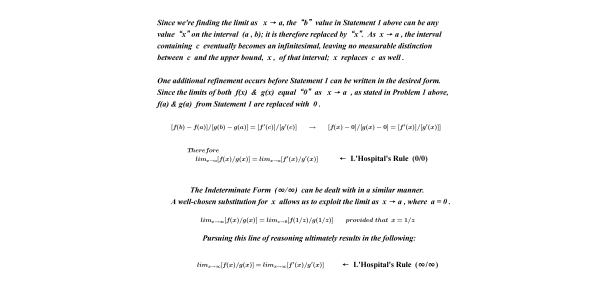
When evaluating limits of rational functions (and others), a minor problem that can arise is the “indeterminate form”, two of which are “0/0” and “∞/∞”.These problems can sometimes be resolved by invoking the Taylor Series, then simplifying from there and evaluating. This, however, can be a time consuming and rather messy process. Another option is to exploit L’Hospital’s Rule, a brief synopsis of which is shown directly below. Several examples of indeterminate forms of limits will then follow.


Mean Value Theorem of Differential Calculus

L Hospitals RuleL Hospitals Rule2


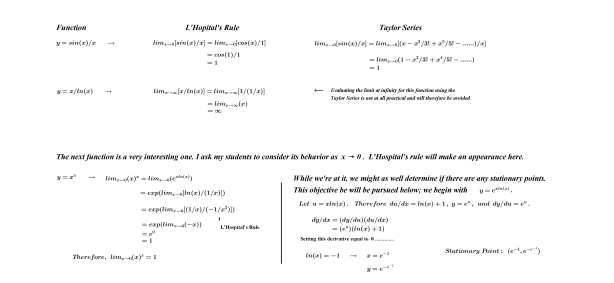
There are four examples below showing the application of L’Hospital’s Rule. The first is the fundamental trigonometric limit that was previously proven using the Squeeze Theorem.

The second example reflects on a previous entry e^(Pi) vs (Pi)^e ; here, the limit as  x →∞  results in the indeterminate form  “∞/∞”.

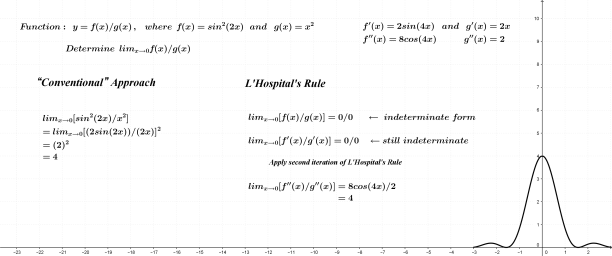
Following e^(Pi) vs (Pi)^e, I’ve included an example illustrating the need for a second iteration of L’Hospital’s Rule. Students can once again practice various rules of differentiation here and, as an added benefit, exploit a trigonometric identity to simplify the process.

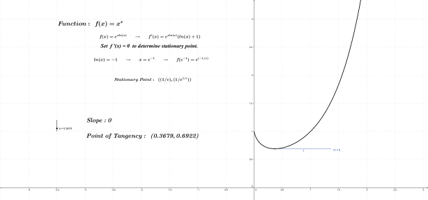
The final example exploits L’Hospital’s Rule in determining the limit of the function  y=x^x  as  x→0. In this scenario, the function itself is tweaked in such a way that leads to an indeterminate limit in the exponent; from this point, L’Hospital’s Rule once again allows us to move forward. The coordinates of this function’s minimum value is also identified to serve as a review of that concept.


Dealing with Indeterminate Limits

Limits L Hospital Taylor Series


Two Iterations of L’Hospital’s Rule

L Hospital's Rule Second Iteration

Click on the link provided here to explore the relationships between y, y’ and y” in  curve sketching.


Graph of f(x)=x^x

x raised to x

Click on the link provided here to explore f'(x) shown in the graph above.


Thanks for reading.


Reference

Kline, Morris.  (1998).  Calculus: An Intuitive and Physical Approach.  Mineola,                             NY:  Dover Publications.


In the spirit of consistency, several additional examples supplementing my introduction to related rates are included here. As seen in the first example below, past concepts are revisited and, in turn, connected to newly introduced ones. Mixing things up from that point on provides students with a variety of perspectives on the same theme that serves to further cement understanding.


Separable Differential Equation

Circle area Derivative


Three Approaches to Related Rates

Circle area Differential Equation


Application to Conical Container

DiffEqua Realted Rates2


Rate of Change of Arc Length

DiffEquaRelatedRatesArcLength


The approach to solving each of these related rate problems is the same; identify what is known, what is desired and then connect the two.


Thanks for reading.

Most related rate problems that high school students see involve three variables. The way in which things unfold usually goes as follows: One rate of change is given, the task being to find another. With three variables in the mix, the typical approach is to find a direct relationship between two of those variables and then express one in terms of the other. The third variable is then be expressed in terms of one variable only, and away we go.

There are cases, however, when all three variables must stand on their own as no direct relationship exists between any two. In such cases, two rates are provided while finding the third rate remains the goal.

The example shown below has a trough filling at a constant rate of 2 cubic feet per minute (dV/dt). The task is to determine the rate at which the depth (height) of water is changing (dh/dt) at any time. Since rates involving volume and height are directly involved here, the typical approach is to express volume in terms of height first and then differentiate. This approach (#1) will follow the image below. Since, however, I like to mix things up and provide alternative ways of thinking, a second approach will be included as well.


The Problem: Determine an expression for dh/dt.


V-Trough2


Approach #1

Related Rates 1

Approach #2

Related Rates 2

The first approach above is more direct in this case. Having said that, awareness of approach 2 will provide leverage to deal with problems in which two independent rates are provided. In those scenarios, the substitution leading to the final expression is not carried out. I included it in the example above to show that each approach yields the same result.

Follow the link provided here to see how the rate of change in depth changes as the trough fills.

Click on the link provided here for more related rates.


Thanks for reading.

Earth-Sun Distance

Posted: February 29, 2016 in Calculus: An Introduction

I was looking through my files last night and came across this. Any ideas about how this could be incorporated into a class activity would be appreciated.

Day-Year

Click on the link provided here to see the Earth’s position relative to the Sun throughout the year.


Thanks for looking.