Archive for the ‘Differential Calculus’ Category

Projectile motion is a natural fit and provides an interesting application in the introduction of calculus at the high school level. A previous post focused on calculating the horizontal velocity of a ball rolling off the end of a table; this entry takes things a bit further by launching projectiles at various angles to determine the maximum horizontal travel.

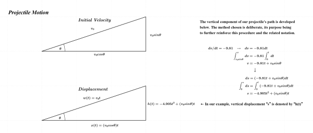
Before lighting the fuse on our launching device, some important theory should first be dealt with. Since our launch angle will be somewhere between 0° and 90°, the projectile’s travel will be directed both vertically and horizontally. Since these values will be dependent on the angle with which the projectile is launched, expressions for distance traveled in terms of that angle will be required. These calculations are shown directly below.

Projections of Velocity

ProjectileMotion1

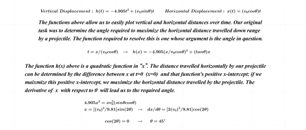
The maximum of the horizontal component of a projectile’s motion occurs when its vertical component has been fully depleted. Since these two conditions occur simultaneously, our work will be straight forward. A new function representing the projectile’s height at any position “x” can be easily determined; x-intercepts of this new function will then lead us to the desired solution.
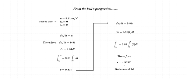
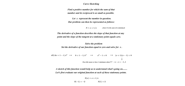
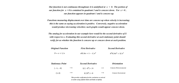
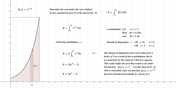
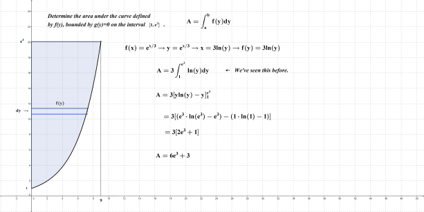
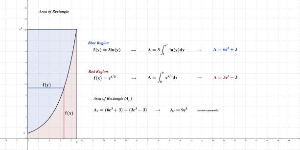
Analytical Solution

ProjectileMotion2

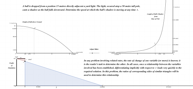
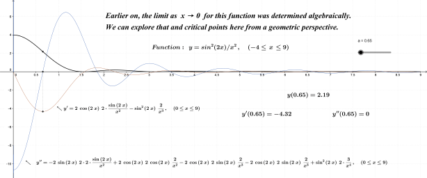
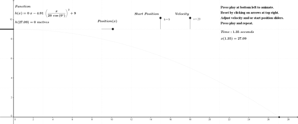
The following is a geometric representation of the analytical solution shown above. The graph on the left shows the projectile’s height as a function of its horizontal position “x”. The second graph measures height over time.

Maximum Horizontal Travel

ProjectileMotion3

Click on the link provided here to interact with projectile motion and discover maximum horizontal travel.

The scenario directly below is supplementary to a previous entry describing a ball rolling off a table. It is included here with the intent of having students further explore the behavior of projectiles launched horizontally from various heights.

Horizontally Launched Projectile

ProjectileMotion4

Click on the link provided here to explore horizontally fired projectiles with  variable height and velocity.

The image and link directly below show how far a baseball would travel with zero drag from air-resistance. The initial launch angle and height have been set to 35° and 1 m respectively. The launch angle can vary greatly and still constitute a baseball scenario; the same cannot be said for the launch height. I decided to leave that variable visible to provide another option for further exploration.

Theoretical Flight of a Baseball (and more)

ProjectileMotionBaseball

Click on the link provided here to explore the path of a baseball assuming zero drag from air-resistance.


The following links verify the accuracy of the model used above and also provide additional insights into the flight of a baseball.

Baseball Trajectory

The Science of Baseball: What Is The Farthest Home Run?

Baseball Physics: Anatomy of a Home Run


Conclusion

Each year, Major League Baseball provides many satisfying projectile launches; the most gratifying (for me) occurred in the 1988 post-season. For a reminder of this moment in time, click on the link provided here to witness what I consider to be the greatest projectile launch of all time……….I love baseball.


Thanks for reading.


Here’s problem involving a falling object and the speed at which its shadow travels along the ground. As usual, in related rates, once a relationship between the variables involved has been established, the calculus required to reach its conclusion is very straight forward.

In order to make efficient use of time, these problems provide students the opportunity to practice simple differentiation procedures. In addition, the graphs provided below open the door to a discussion on the Mean Value Theorem of differential calculus, serving to either introduce or reinforce that concept.


Falling Ball

RelatedRatesBallDrop

Click on the link provided here to interact with the falling ball and its shadow.


The ball’s displacement from its release point was provided in the image above. As a review (since integral calculus has already been introduced), that displacement formula is once again derived through basic differential equations; this is shown directly below.

Acceleration, Velocity and Displacement

BallDropDisplacementFormula


I’ve included solutions for  t=1  and  t=2  below. In keeping with my belief that students can learn effectively through comparison and contrast, three varied methods are shown.

Solutions

RelatedRatesBallDropSolutions

Thanks for reading.

The main subject of this entry was originally planned as an optimization problem involving differential calculus only; its been slightly modified. This more interesting approach provides the derivative up front, presenting students with three separate tasks to pursue from that point. As a consequence, students are reintroduced to differential equations and curve sketching.

A talking point emerges as well: Is there a difference between derivatives and differential equations?


Inscribed Triangle of Maximum Area

Inscribed Triangle animation


Click on the link provided here to explore area of the inscribed triangle.


Thanks for looking.

By the time curve sketching is formally introduced, students have already seen a few “purposeful” examples; they are listed below as links.

Putnam Problem, Four Townse^(Pi) vs (Pi)^ef(x)=x^x (L’Hospital’s Rule)

Through these examples (and others), first and second derivatives have been points of discussion with respect to identifying the location and nature of critical points. In addition to this, L’Hospital’s Rule will have been established along the way and thrown into the mix.

My formal introduction to curve sketching is introduced in the form of a problem solving scenario. An example of this is shown below.


Sum of a Number and its Reciprocal

Curve Sketching


Limits at Infinity & Infinite Limits

Curve Sketching2


First and Second Derivatives

Curve Sketching3


Graph of   S(x) = x + 1/x

x + 1 by x

Click on the link provided to interactively determine the local extrema.


Graph of   y=sin^2(2x)/x^2  (see L’Hospital’s Rule for indeterminate limits of this function)

L Hospital's Rule Second Iteration2

Click on the link provided here to explore the relationships between  y, y’ and y”.


Thanks for reading.

In the spirit of consistency, several additional examples supplementing my introduction to related rates are included here. As seen in the first example below, past concepts are revisited and, in turn, connected to newly introduced ones. Mixing things up from that point on provides students with a variety of perspectives on the same theme that serves to further cement understanding.


Separable Differential Equation

Circle area Derivative


Three Approaches to Related Rates

Circle area Differential Equation


Application to Conical Container

DiffEqua Realted Rates2


Rate of Change of Arc Length

DiffEquaRelatedRatesArcLength


The approach to solving each of these related rate problems is the same; identify what is known, what is desired and then connect the two.


Thanks for reading.

Most related rate problems that high school students see involve three variables. The way in which things unfold usually goes as follows: One rate of change is given, the task being to find another. With three variables in the mix, the typical approach is to find a direct relationship between two of those variables and then express one in terms of the other. The third variable is then be expressed in terms of one variable only, and away we go.

There are cases, however, when all three variables must stand on their own as no direct relationship exists between any two. In such cases, two rates are provided while finding the third rate remains the goal.

The example shown below has a trough filling at a constant rate of 2 cubic feet per minute (dV/dt). The task is to determine the rate at which the depth (height) of water is changing (dh/dt) at any time. Since rates involving volume and height are directly involved here, the typical approach is to express volume in terms of height first and then differentiate. This approach (#1) will follow the image below. Since, however, I like to mix things up and provide alternative ways of thinking, a second approach will be included as well.


The Problem: Determine an expression for dh/dt.


V-Trough2


Approach #1

Related Rates 1

Approach #2

Related Rates 2

The first approach above is more direct in this case. Having said that, awareness of approach 2 will provide leverage to deal with problems in which two independent rates are provided. In those scenarios, the substitution leading to the final expression is not carried out. I included it in the example above to show that each approach yields the same result.

Follow the link provided here to see how the rate of change in depth changes as the trough fills.

Click on the link provided here for more related rates.


Thanks for reading.

Now that the formula for arc length has been determined, we can pursue surface areas of curved solids.

Some students have great difficulty conceptualizing areas on curved surfaces. The problem lies in the fact that they want to use Δx or Δy in the setup, just as they did when calculating volumes of solids and areas over flat surfaces. Since on a curved surface, both x and y are changing in unison; as one changes, so does the other. For this reason, we need to use a variable linking those two variables together. This brings into play the Pythagorean Theorem and arc length. Arc length is a one-dimensional measure, its formula the result of capturing the interplay between Δx and Δy and expressing that as Δs. Integrating the one-dimensional Δs over a given interval will therefore produce the desired outcome (even though the path might not be linear, its distance is nevertheless one-dimensional).

A similar argument can be made for calculating areas over curved surfaces. Since area is two-dimensional, the integral we set up to calculate area must stick to that. I visualize a sphere wrapped with very narrow “bands”. If one of these bands was removed and cut, it could be stretched out and laid flat; its length on one edge would exceed that of the opposing edge due to the fact that it was wrapped around a curved surface. Ultimately this is not a problem, however, since these two opposing edges approach the same length as the distance between them narrows. This is entirely similar to each annulus in a previous post where circle area was derived using the “onion proof“.

This takes care of one dimension required for surface area. The second dimension is arc length mentioned in paragraph two above. As  Δs approaches zero, the line segment joining the two infinitely close points that determine the “point” of tangency becomes ever more perpendicular to the length of each band mentioned earlier. Each band can be treated as a rectangle; area is determined as the product of width (arc length) and length (circumference of 3-D solid) at each x_i over the given interval.


The following notes reveal surface area of a sphere using the reasoning described above.

Sphere

Surface Area (sphere)Conventional

Click on the link to view the changing width of each “band” around the sphere.


As before, students can once again benefit having a second example from which to draw comparisons to the first; the cone serves this purpose very well.

Lateral Surface Area of Cone

Cone Lateral Area


Thanks for reading.

For the past week or so, we’ve been focused primarily on differential calculus and becoming comfortable with the rules that have been derived through the limiting process. The derivatives of e^x and ln(x) were both derived but only the anti-derivative of the former reveals itself through that process. Since the primitive of ln(x) remains a mystery, only the first part of the exploration below can be tackled.

In order to facilitate completion of the entire sequence below, I will ask the students to determine the derivative of f(x)=-x+xln(x). The result will be very useful for our purposes here and will also launch us into Integration by Parts.

AreaUnder exp


AreaUnder exp2


AreaUnder exp3


Thanks for reading.

Having previously determined the derivative of ln(x), we now have that at our disposal to show one perspective of the product and quotient rules of differential calculus. A quick excursion to “implicit differentiation land” and a review of the chain rule will set things up nicely to meet our objectives here.

Implicit Diff and Chain Rule


Product and Quotient Rules

Product Quotient Rules

Modified Product Rule

Modified Product Rule

Thanks for reading.

Once students have a feel for calculating derivatives by limits of various functions, the same is done for ln(x) and e^x. Each of these show the importance of binomial expansion as that skill is once again necessary in understanding why things are as they are.

Derivative of ln(x)

Derivative(ln)

The derivative of ln(x) have many applications including logistic growth which we will see later this semester. We can, however, put this to work immediately by using it along with our knowledge of the product and quotient laws of logarithms. These are woven together nicely to determine the product and quotient rules of differential calculus.

The Euler constant “e” is also exploited in deriving the Rule of 72.


Derivative of e^x

Derivative(e^x)


Geometric Perspective of d(a^x)/dx

Derivative Exponential Function

To interact with the function above, click on d(a^x)dx.

Click the link provided to see two additional perspectives on the derivative of e^x.


Thanks for reading.


Reference

Courant, Richard., John, Fritz (1999).  Introduction to Calculus and Analytics: Classics of Mathematics. New York, NY:  Springer-Verlag Berlin Heidelberg.