Posts Tagged ‘Differential Equations’

Here’s problem involving a falling object and the speed at which its shadow travels along the ground. As usual, in related rates, once a relationship between the variables involved has been established, the calculus required to reach its conclusion is very straight forward.

In order to make efficient use of time, these problems provide students the opportunity to practice simple differentiation procedures. In addition, the graphs provided below open the door to a discussion on the Mean Value Theorem of differential calculus, serving to either introduce or reinforce that concept.


Falling Ball

RelatedRatesBallDrop

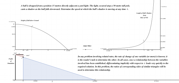
Click on the link provided here to interact with the falling ball and its shadow.


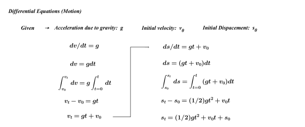
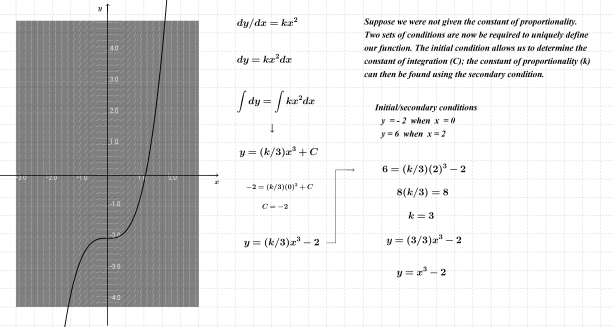
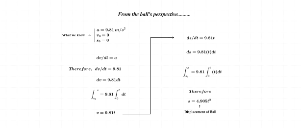
The ball’s displacement from its release point was provided in the image above. As a review (since integral calculus has already been introduced), that displacement formula is once again derived through basic differential equations; this is shown directly below.

Acceleration, Velocity and Displacement

BallDropDisplacementFormula


I’ve included solutions for  t=1  and  t=2  below. In keeping with my belief that students can learn effectively through comparison and contrast, three varied methods are shown.

Solutions

RelatedRatesBallDropSolutions

Thanks for reading.

Having side-by-side comparisons can be valuable experience as similarities (and differences)  are more readily apparent; students can gain a deeper understanding of the nuances from one to the next. For example, its worth noting that the rate of change of a circle’s area with respect to its radius is equal to that circle’s circumference; a similar relationship exists between the volume and surface area of a sphere.

Investing some thought into these and other subtleties can go a long way towards increasing one’s intuitive feel for, and enjoyment of this discipline.

DiffEqua(Constant,Linear,Quad)

Another comparison worth checking out is quadratic vs exponential growth.

Thanks for reading.

I, like most others, always attempt to use students’ existing knowledge base on which to build and connect new concepts (or new perspectives on old concepts); simple motion problems are one such example. The concept in this entry is integration and it provides a new and very rich perspective on an “old” concept already familiar to students.


The following excerpt is taken from reflections of my 1st two weeks in calculus.
Question: What can we do when “dv=(a)dt” shows up in this way?
Answer: We can integrate.
Question: What does integration give us?
Answer: The area between the function and the x-axis.
Question: What does our function represent?
Answer: Acceleration.
Question: What does the area in question represent?
Answer: Velocity.
Question: Have you ever seen this before and, if so, where?
Answer: Yes, in Physics class.


DiffEquations (Motion)2

As an extra activity, students could sketch slope fields for dv/dt and ds/dt to become more familiar with those. In addition, students would also benefit from drawing comparisons between integrating functions in 2-dimensions above (focus on area) and its 3-dimensional counterpart.

Thanks for reading.

In order to achieve some degree of continuity, I continually strive to weave together concepts, not only within my own “area of influence”, but across other disciplines as well. Physics is naturally folded into the fabric of calculus for obvious reasons; others disciplines, not so much.

I wanted to raise awareness in students of how calculus appears in applications relating to Biology and Chemistry; logistic growth is the obvious choice for the former and is relatively straight forward once students have a feel for differential equations.

The notes directly below make clear (I hope) the distinction between two types of growth from the context of differential equations.  The exponential growth model below will be expanded upon to eventually derive the well-known formula for logistic growth.

Separable Diff Equations2


The application to Chemistry that was alluded to earlier will require First Order Differential Equations, another “diversion” that can be pursued when a change of pace is needed. We will hopefully be afforded the time to develop an adequate understanding of this before semester’s end.

Thanks for reading.

A basic understanding of differential equations has already been established through our introduction to integration. In addition, rates of change have also been linked to our brief study of differential calculus. Students now require a period of time to work through basic problem solving scenarios relating to both differentiation and integration to develop an acceptable degree of fluency.
Every now and then, a diversion from the “daily grind” can be well-received. Separable differential equations and an introduction to slope fields will be one such “diversion” and will be shared with students when deemed appropriate. Since students are very familiar with quadratic functions, will we begin there.
The equation dy/dx=x will be presented and analyzed from a “rate of change” perspective at various positions on the Cartesian plane. Once this slope field has been sketched, the shape of the parent function becomes readily apparent; the need for initial conditions arises to uniquely define each member from the family.
The image directly below sees through the completion of the scenario described above. This procedure is then repeated for other basic separable differential equations, all of which produce slope fields that are recognizable to students; these appear below our parabola example.


Differential Equation: dy/dx=kx, where k=2

Constant of Proportionality Given

Quadratic 2x(2)


Differential Equation: dy/dx=kx^2, where k=3

Constant of Proportionality Given

Cubic 3x^2 (2)


Constant of Proportionality Not Given

Cubic 3x^2(3)


Differential Equation: dy/dx=-x/y

Circle -x over y (2)

For the circle above, I’ve included two acceptable treatments.

The indefinite integrals require that initial conditions be substituted in after the fact to solve for the constant of integration.  The second version has the initial conditions included as bounds of integration, resulting in definite integrals; same result.


Solving these differential equations tie together quite nicely the two sides of calculus to which students have been introduced. These examples also set up other such equations and problems that will be presented in the not too distant future, such as  Quadratic vs Exponential Growth.

Thanks for reading.