samuelson mathxp

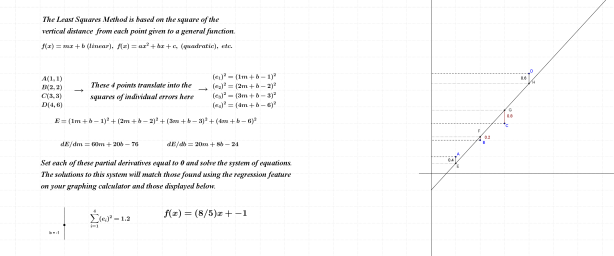
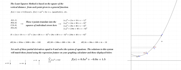
The question I pose to students in Introductory Calculus might take on the following form:

A really REALLY REALLY long ship is sailing parallel to a shoreline, 2 km off shore. A lighthouse on the shore projects its beam in a circle; the angular velocity at the point of rotation is given. Determine the linear velocity, from the lighthouse keeper’s perspective, of the beam’s leading edge as it passes by the ship from stem to stern as the ship sails on.  Then consider another scenario; the ship’s frisky dog can run 30 km/h.  Determine the beam’s angular velocity that would allow the dog to keep up to its leading edge as it sweeps past the length of the ship under the following conditions:

(a) the ship is 2 km off shore and positioned at 60 degrees East of North relative to the lighthouse.

(b) the ship is 500 metres off shore at 60 degrees East of North relative to the lighthouse.

(c) the ship is 500 metres off shore due north of the lighthouse.

Although this example is obsolete with the advent of GPS, the mathematics in it is not. This is a very effective “end game” to pursue for students in Introductory Differential Calculus as it requires them to find the instantaneous velocity at a specific point. In fact, many such velocities could be determined from the perspective of an observer on the ship, connecting each to the relative position on the accompanying sinusoidal function……..when is that velocity positive, negative, etc……

The math learned in this example could be applied in the same way to many other similar scenarios.  I will be developing meaningful lessons over the course of the next several weeks, the purpose of which is to empower those taking an interest in solving the problem above……..and many many more.  They will be hand-written and saved as photo files; links to those notes will be added below as they become necessary.

POWER RULE

A good amount of work must be accomplished before we can get to the solution of our light house problem.  To get started, I have written eight pages of notes introducing the notion of derivative using first principles.  To view those notes, click on the link below. 

First Principles (Polynomial & Radical Functions) – Samuelson

The notes found in the link above made reference to the factorization of a difference of cubes shown below:

x^3 – 27 = (x – 3)(x^2 + 3x + 9)

I will illustrate a very powerful method of factoring such things; this method is based on a geometric representation of the factoring problem.  The original difference of cubes (or sum of cubes) represents the area of a rectangle; the factors of that become the side dimensions of said rectangle.  I came across a “gold mine” of information recently in which this method of factoring is included.  James Tanton has put forth a vast collection of video lessons on YouTube to help students and teachers alike to better understand mathematics.  The link below takes you to one such lesson describing the factoring method to which I refer.

James Tanton: Synthetic Division: How to understand it by NOT doing it! (VIDEO!)

The following link contains notes showing more examples of Tanton’s division.  These examples ultimately lead to a deductive proof of the power rule for finding derivatives; read through carefully.

Proof of Power Rule – Samuelson

Our lighthouse problem represents cyclic motion; the function describing this will therefore be a sinusoidal function, perhaps represented by  y=sin(x).   Since we are asked to determine instantaneous velocity at a given point, the derivative of the function will be required.  The four pages of notes found in the link below describe the process of finding that derivative.

Fundamental Trig. Limits – Samuelson

PRODUCT, QUOTIENT & CHAIN RULES

The last thing we need in place so that we can solve our lighthouse problem is the “Chain Rule”.  You’ve already seen the Power Rule and its proof; this rule is inherent in all of Differential Calculus and, as such, will be utilized within the Chain Rule as well.  Clicking on the link below will take you to notes describing this rule and two others; the Product Rule and the Quotient Rule.  I will post examples using these rules to find derivatives of various functions at a later date.

Product, Quotient & Chain Rules – Samuelson

We are getting ever closer to a meaningful solution to the lighthouse problem presented at the outset; the underlying logic behind this solution is very simple.  Several rules have been introduced and proven (hopefully to your satisfaction) and the concept of instantaneous velocity should now be firmly entrenched in your thought process.  In the notes below, I have given a few examples of functions; the differentiation rules are illustrated there in finding the correspnding derivatives.  I’ve also taken this opportunity to introduce “acceleration” from a “derivatives” perspective.

Applications of First & Second Derivatives – Samuelson

IMPLICIT DIFFERENTIATION & RELATED RATES

The notes contained in the link directly below introduce you to Implicit Differentiation and Related Rates; these rate problems will typically involve three variables, one of which is “time”.  Our lighthouse problem is, itself, a related rate and can be solved through the explicit process.  Having said that, the implicit procedure lends itself in a more consistent manner to a wide range of related rate problems.  Consequently, I thought it appropriate to describe that process at this time and provide examples of its use in solving several related rate problems.  These examples will provide the remaining tools required in completing your task.

Implicit Differentiation & Related Rates – Samuelson

Additional links for reference purposes are found below.

Implicit Differentiation

Related Rates

The solution to our lighthouse problem is shown on page 6 of the notes contained in the link directly below.  A description of how angular and linear velocity relate to one another occurs in the pages preceding that.  A firm understanding of this will enable you to reason your way to solution to all such “problems” in a much more meaningful way.

Angular & Linear Velocity – Samuelson

Our lighthouse problem has now been solved.  The procedures and thought patterns established through this process can be applied in the same manner to set up and solve many such problems; I may add some of those to this page at a later date.  For now, I will turn my attention to Integral Calculus; my goal in this will be to derive the arc length of a circle of given radius.

Please visit  James Tanton, The Republic of Math and Cut The Knot for all things related to Mathematics.

As a footnote to our exploration above, the link below may be of interest.

Superluminal Motion