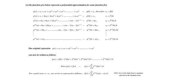
Suppose we would like to approximate a function f(x) by some simpler polynomial function g(x) near some value “x=a” (radius of convergence). The result is referred to as the Taylor Series (or Taylor expansion) of the function f(x).
To keep things tidy, the examples here will involve polynomial approximations of f(x) near “x=0”. The constant term (y-intercept) of the original function f(x) and its polynomial approximation are easily determined; it would simply be “f(0)”. It stands to reason that the slopes of the functions in question must be equal to one another at “x=0″ as well. Hence, f'(0) must therefore equal to g'(0). The same argument holds true for the second, third, fourth derivatives and so on. Our goal is to represent the parameters of g(x) in terms of f(0), f'(0), f”(0), etc.
The result of the process outlined above is called the “Taylor Series”. The template for this series will be fleshed out below and then applied to several well-known functions to arrive at their polynomial approximations.
Taylor Series Derived
Applying any new concept and comparing with what is already known is always good practice. Below, the Taylor expansion is applied to three functions that are very familiar to high school students. The links that follow provide students the opportunity to interact and explore how the Taylor Series behaves as “n” increases without bound.
e^x, sin(x) and cos(x)
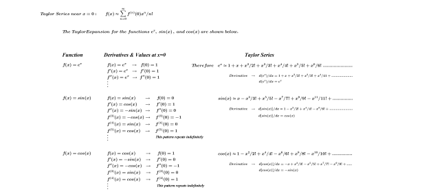
Click on the following links to explore each function.
f(x)=e^x , f(x)=sin(x) , f(x)=cos(x)
Having seen the Taylor expansion for the three functions above, the stage is now set up very nicely to bring this entry to its conclusion.
Euler’s Formula

Thanks for reading.
Reference
Courant, Richard., John, Fritz (1999). Introduction to Calculus and Analytics: Classics of Mathematics. New York, NY: Springer-Verlag Berlin Heidelberg.

