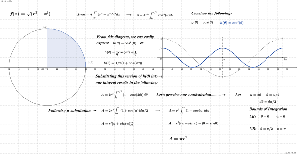
When working with composite functions, u-substitution often simplifies the integration process for us. What is sometimes overlooked, however, is the significant adjustment that occurs to the area beneath the curve.  The image and link below allow students to explore the significance of this procedure.

ChainRule Area Cos

Interactively explore u-substitution.


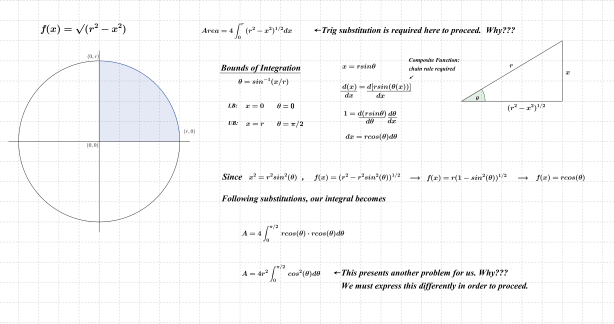
As seen below, u-substitution is not a viable approach to integration as its leads to division by zero. In the case below, and others like it, trigonometric substitution provides a means for us to move forward and solve many problems. The process below also brings trigonometric identities into play, thereby  exposing students to their significance.

Circle Area Trig Substitution Formula1

Circle Area Trig Substitution Formula2

Thanks for reading.

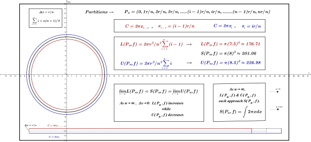
As I’ve stated before, circle area would once again be investigated. This iteration brings uniform sub-intervals into play (apologies for all the color but thought it would be helpful for students to distinguish upper and lower bounds).  The link directly below this image opens a new tab from which students can adjust two parameters to explore the partitions; those sliders appear at the right-hand side near the bottom.

Circle Area(2)BLOG

In the image above, there are two rectangles displayed; the length of the blue rectangle is based on the circumference of the upper bound, the length of the red on the lower bound. By reducing the width of each partition (link below), you will see that these two lengths approach a common value.

Interactive exploration of the image directly above.


Circle Proof (Uniform)


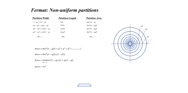
For a direct comparison between this version and that using non-uniform partitions, I’ve added the image below.

Fermat Circle

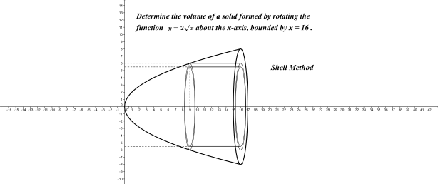
One final note here: Area of the circle using annuli of uniform sub-intervals extends naturally to volumes by cylindrical shells. Walls extend perpendicular to the upper and lower bounds of each annulus; the height of these walls is governed by a function of “x” (single variable calculus). For f(x)=c, the layering effect of cylindrical shells forms a cylindrical solid. For f(x)=ax+c, the solid formed is a cone, if f(x)=ax^2+b, a paraboloid emerges. These are a reasonable conclusions that high school students readily accept. Volumes by slabs follow the same argument. 

Cylindrical Shells

Volume Cone Shells4

I also like to have students set up integrals from both dx & dy perspectives (as seen below).

Paraboloid (shells)


Thanks for reading.

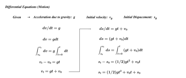
I, like most others, always attempt to use students’ existing knowledge base on which to build and connect new concepts (or new perspectives on old concepts); simple motion problems are one such example. The concept in this entry is integration and it provides a new and very rich perspective on an “old” concept already familiar to students.


The following excerpt is taken from reflections of my 1st two weeks in calculus.
Question: What can we do when “dv=(a)dt” shows up in this way?
Answer: We can integrate.
Question: What does integration give us?
Answer: The area between the function and the x-axis.
Question: What does our function represent?
Answer: Acceleration.
Question: What does the area in question represent?
Answer: Velocity.
Question: Have you ever seen this before and, if so, where?
Answer: Yes, in Physics class.


DiffEquations (Motion)2

As an extra activity, students could sketch slope fields for dv/dt and ds/dt to become more familiar with those. In addition, students would also benefit from drawing comparisons between integrating functions in 2-dimensions above (focus on area) and its 3-dimensional counterpart.

Thanks for reading.

Grade 10 class would be split into two groups. Each group would then select a linear function and determine 3 ordered pairs that satisfy their function.

Those ordered pairs would be handed off to Math 31 students who would then use Method of Least Squares and partial differential equations to develop a system of linear equations in two variables for each set of points they received.

These systems of linear equations would then be sent back to the Grade 10 class to the opposing group. The solution to each system would reveal the parameters from the original function of the rival gang. Members would then “guess” the original equation of the other group.


The same “contest” would occur between Grade 11’s and Math 31. This time, however, quadratic functions would be the subject and 4 ordered pairs produced for each group.  The systems of equations received back from Math 31 would be quadratic in nature, containing three variables.


Thanks for reading; comments appreciated.

In order to achieve some degree of continuity, I continually strive to weave together concepts, not only within my own “area of influence”, but across other disciplines as well. Physics is naturally folded into the fabric of calculus for obvious reasons; others disciplines, not so much.

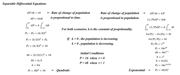
I wanted to raise awareness in students of how calculus appears in applications relating to Biology and Chemistry; logistic growth is the obvious choice for the former and is relatively straight forward once students have a feel for differential equations.

The notes directly below make clear (I hope) the distinction between two types of growth from the context of differential equations.  The exponential growth model below will be expanded upon to eventually derive the well-known formula for logistic growth.

Separable Diff Equations2


The application to Chemistry that was alluded to earlier will require First Order Differential Equations, another “diversion” that can be pursued when a change of pace is needed. We will hopefully be afforded the time to develop an adequate understanding of this before semester’s end.

Thanks for reading.

A basic understanding of differential equations has already been established through our introduction to integration. In addition, rates of change have also been linked to our brief study of differential calculus. Students now require a period of time to work through basic problem solving scenarios relating to both differentiation and integration to develop an acceptable degree of fluency.
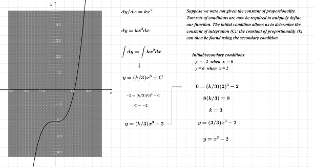
Every now and then, a diversion from the “daily grind” can be well-received. Separable differential equations and an introduction to slope fields will be one such “diversion” and will be shared with students when deemed appropriate. Since students are very familiar with quadratic functions, will we begin there.
The equation dy/dx=x will be presented and analyzed from a “rate of change” perspective at various positions on the Cartesian plane. Once this slope field has been sketched, the shape of the parent function becomes readily apparent; the need for initial conditions arises to uniquely define each member from the family.
The image directly below sees through the completion of the scenario described above. This procedure is then repeated for other basic separable differential equations, all of which produce slope fields that are recognizable to students; these appear below our parabola example.


Differential Equation: dy/dx=kx, where k=2

Constant of Proportionality Given

Quadratic 2x(2)


Differential Equation: dy/dx=kx^2, where k=3

Constant of Proportionality Given

Cubic 3x^2 (2)


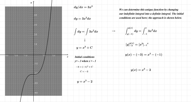
Constant of Proportionality Not Given

Cubic 3x^2(3)


Differential Equation: dy/dx=-x/y

Circle -x over y (2)

For the circle above, I’ve included two acceptable treatments.

The indefinite integrals require that initial conditions be substituted in after the fact to solve for the constant of integration.  The second version has the initial conditions included as bounds of integration, resulting in definite integrals; same result.


Solving these differential equations tie together quite nicely the two sides of calculus to which students have been introduced. These examples also set up other such equations and problems that will be presented in the not too distant future, such as  Quadratic vs Exponential Growth.

Thanks for reading.

First Week

Day 1
The branch of mathematics called “calculus” was defined as the “mathematics of change”. A discussion of the movement of a point residing on the Earth’s equator and the corresponding position function was determined. Slopes of this function at the critical points were determined, interpreted and compared to a second function (derivative of the displacement function). With the help of technology to determine slopes, connections quickly became apparent between rates of change of the displacement function with respect to time and the value of the second function. Students immediately wanted to know more and were informed that they would soon learn an efficient method of determining rates of change.

Buffon’s experiment was also recreated and an estimate for π emerged. I mentioned to students that the reasoning behind this method will be constructed by the middle of March (π week). Students were also informed that probability and calculation of areas would be required to meet this challenge.

The two branches of calculus had now been introduced within the first 40 minutes of our 80 minute block. Following a very brief discussion of what Newton and Leibniz contributed to mathematics, the students were primed to further investigate either branch.
It was decided that we would spend the remainder of our class time investigating the volume of a cone. The formula for sum of triangular numbers was quickly determined; this was followed by a more lengthy derivation of the formula for sums of squares (using telescoping sums). With these in place, a linear function having slope r/h was drawn through the origin. I asked the students to imagine what shape would emerge if we could rotate that line around the x-axis; a cone was visualized and notion of volumes of revolution introduced. I quickly sketched a cross-sectional slab of thickness ∆x; this cylindrical slab was duplicated away from the cone and its volume was quickly identified. Discussion ensued with respect to similar cross-sectional slabs cut from other positions on the cone; students immediately noticed that the radius varied and was governed by the linear function f(x)=(r/h)x.

Students quickly agreed that by calculating volumes of individual slabs and summing (integrating) those on the interval [0, h], a reasonable estimate for the cone’s volume should emerge. Uniform sub-intervals of length ∆x=(h/n) were then established and recorded on the white board. Students accepted the idea that if “n” were to increase without bound, the cylindrical slabs would become increasingly narrow and the estimate for the cone’s volume would become more precise.

It was then decided that the radius of each slab “f(x)” could be based on the upper bound of each sub-interval (since all values of ” x ” from there to the lower bound become infinitely close to one-another as “n” increases without bound). Following some factoring, an appropriate substitution of the sum of squares formula and evaluation of limits as “n” moves to an infinitely large value, the well-known formula for volume of the cone appeared; minds blown (in a good way).

We will soon turn the cone onto its base and calculate volume by horizontal slabs (as shown directly below) and eventually by cylindrical shells (lower image).

Horizontal Slabs
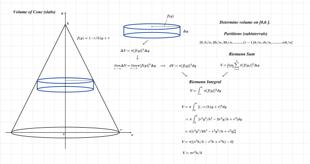
Volume of Cone (slabs)


Cylindrical Shells

Volume Cone Shells4


Later in the week, the power rule for integral calculus was derived using Fermat’s non-uniform sub-intervals as shown in the image below; the Fundamental Theorem of Calculus was also established at this point. The cone’s volume was once again derived by adding volumes of slabs sliced from uniform sub-intervals. Students now discovered that these discrete volumes (Riemann sums) gave way to their continuous counterpart (Integral). Applying the power rule of integration to π((r/h) x)^2 and evaluating the result over the interval [0, h] using the FTC quickly produced the desired formula. The integral notation was adopted soon thereafter.


Fermat’s Non-Uniform  Partitions
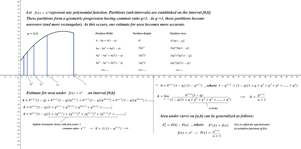
Fermat

The time remaining over the final two days of Week 1 primarily involved students setting up and evaluating integrals; primitives of functions for which the power rule did not work were provided as the assignment given included those as well. The primitives of these functions will later be determined and defined further as anti-derivatives through the use of differential calculus.


Second Week

Day 1

A review of the previous week’s topic was followed by the introduction of rates of change. The introduction of a new topic always involves discussion and students are asked to avoid note-taking; engagement in discussion, diagrams and analysis is maximized in this way. What is learned on day 1 will be summarized with carefully scripted notes the following day (discussion is always included here as well for clarification when needed).

The function f(x)=x^2 was used initially with a secant line drawn between two distinct points P and Q. An expression for the slope of this line (average rate of change) was determined for “x” and “(x+∆x)”. A right triangle was then sketched and the slope of the line segment PQ was related to the tangent ratio of the angle formed at point P. It was then determined that the tangent line at P would become the limiting case of secant PQ (since ∆x can never be zero). A direct comparison to points of discontinuity from Math 30 was also made here. We will discuss left- and right-hand limits to determine whether or not a function is differentiable at a given point later on this semester; it is an unnecessary distraction at this point.

Preceding the delivery of my notes on day 2, the drill from the previous day was repeated, this time with f(x)=x^3. When comparing the results from the two functions, a pattern seemed to have emerged. Having seen this limiting process twice, the notes on differential calculus would now have some meaning to students. The term “derivative” was introduced and shown that it is itself a function. Various notations of the derivative were also introduced here (Leibniz, Lagrange, Newton) as were numerical representations. Several examples of f'(x) and f'(a) were worked through in class together and then time given for students to practice.

When students need a break from practice, I give them something new to think about. On day 3, we brought some simple physics into play. Students already know that acceleration is the rate of change of velocity with respect to time; dv/dt=a. Since they learned simple differential equations in week one, the equation above was re-written as dv=(a)dt.

The following exchange ensued:
Question: What can we do when “dv=(a)dt” shows up in this way?
Answer: We can integrate.
Question: What does integration give us?
Answer: The area between the function and the x-axis.
Question: What does our function represent?
Answer: Acceleration.
Question: What does the area in question represent?
Answer: Velocity.
Question: Have you ever seen this before and, if so, where?
Answer: Yes, in Physics class.
Comment: Now you know why Newton invented calculus!

Getting back to our differential equation…….
The process of integration above resulted in v=at+v_0.
We then executed the same process once again, this time for ds/dt=v.
Repeat question/answer sequence.

Through the integration of ds=(at+v_0)dt, the displacement function encountered so many times in Math 20-1 (and Physics 20) appeared.

s=(a/2) t^2+(v_0) t+s_0

This happens very quickly and gets students thinking. It also brings back the topic of integration and sets up very nicely the inverse relationship between derivatives and integrals.


Other “extras” that were thrown in during week 2:
-Chain Rule using Leibniz notation and “u”substitution.
-proof of fundamental trig limits
-derivative of sin(x) through algebraic analysis and graphing

Additional information given but not yet derived:
-product rule: d(fg)=f’g+g’f
-quotient rule: d(f/g)=(f’g-g’f))/g^2
– d/dx ln(x)=1/x

– d /dx cos(x)=-sin(x)……this was reasoned out using graphs.


Upcoming:
-derivatives of ln(x),e^x,cos(x) and proofs of product & quotient rules using logarithms.

-setting up and solving simple differential equations from slope fields

-further analysis of significance of chain rule as it applies to derivatives AND integrals. This analysis will occur both geometrically and analytically.

-linear regression using method of least squares.

By the end of February, students will be quite fluent in setting up and solving simple problems involving derivatives and basic integrals. Further work with limits and curve sketching will be done later in the semester and will seem trivial by that time.

It is clear from this entry that I am a “constructivist”. I realize that some proponents of discovery learning will hammer on me for this; that is fine. There is still plenty of room in this approach for students to explore and discover connections on their own. Differentiation and integration are tools for other pursuits, not an end in themselves. This not meant to insult high school math students but it would take them much longer than 2 weeks to be in the position we presently find ourselves.

Between now and the end of this semester, we will continue to explore circle area, cone volume, arc length, etc. and through those pursuits, trigonometric substitution, integration by parts and partial fractions will eventually emerge; the proof of Buffon’s needle experiment in the middle of March will seem anti-climactic. Logistic growth, work, centers of mass in 1- & 2-dimensions, and other more complex applications of calculus will also be pursued and tackled.

That’s all I have to say for now.
Thanks for reading.


Reference:  Courant, Richard., John, Fritz (1999).  Introduction to Calculus and Analytics: Classics of Mathematics. New York, NY:  Springer-Verlag Berlin Heidelberg.

I’ve always liked using the “onion proof” as an easy approach to showing students why the area of a circle is what it is. I also strive to fold in as many previously learned concepts as possible when introducing new ones.  Fermat’s non-uniform partitions provide a very rich approach to deriving areas.  This approach as it applies to the circle is shown directly below.  As you will see, factoring skills that students have learned in Grades 10 and 11 are put to work and out pops the circle’s area; students like this.


The Setup

A line on [0,1] was first drawn, then partitions based on q=0.5 identified; those partitions were then summed and the total approached 1 (as it should). This idea was then connected to the formula for sum of infinite geometric series (which was also quickly derived). Additional iterations with q=0.9 and q=0.99 revealed that the non-uniform partitions would become “more uniform” as “q” approached “1”. This idea was then generalized over the interval [0,r] and the lengths of each sub-interval determined.

Concentric circles were eventually drawn around the lower bound of the main interval and the area of each annulus was reasoned out through discussion. It was concluded that the upper bound of each sub-interval could be used to represent the length of each annulus, with the span of the corresponding partition equal to its width. It was agreed upon that these annuli, when”sliced” and “unrolled”, formed rectangles whose areas were easily determined.
Lengths, widths, and ultimately areas of at least 3 of these rectangles were recorded and then summed. Some simple factoring revealed a “new” expression with recognizable components. After some simplification, “q” was replaced with “1” and out popped a very good estimate for the area of a circle.
This process was then repeated for f(x)=x^2 and f(x)=x^3 since the factoring skills required for those was also in place. The entire process was then generalized and applied to the function f(x)=x^n and from this, our expression F(x) was determined.

Shown below are the circle and f(x)=x^n. The links provided here allow students to adjust the common ratios for each and view the resulting partitions.

Non-Uniform Partition Exploration: Circle

Fermat Circle

If we were to sketch a function of area “A” with argument “q”, we would find that it has a point of discontinuity at (1,  πr^2). We can say that the function has a limit of  πr^2 as “q” approaches 1.


Non-Uniform Partition Exploration: f(x)=x^n

Fermat

Thanks for looking.


Reference

Courant, Richard., John, Fritz (1999).  Introduction to Calculus and Analytics: Classics of Mathematics. New York, NY:  Springer-Verlag Berlin Heidelberg.

As stated in my previous entry, I like introducing Calculus from the Integral side. My students are already familiar with areas of circles and volumes of cylinders but curiosity still persists with respect to why the volume of a cone is what it is.  The first two days are thus surrendered to discussion revolving around this topic.

Sigma notation is first discussed and the formula for sum of triangular numbers is quickly derived.  I also mention that the formula for sum of squares is required in our search for the cone’s curious volume.  They want to see how it is derived; enter telescoping sums.  Through these procedures, students are introduced to new notation and gain insights into how concepts they’ve already learned are exploited in the search for bigger things.

Once the sum formulas are in place, the interval [0,h] along the x-axis is divided into sub-intervals of uniform length.  This length determines the “height” dimension of each cylindrical slab; the radius is based on the upper bound of each partition.  It is clear to all that this radius is variable and is governed by f(x).  After some scribbles and factoring, the need for sum of squares formula surfaces and soon thereafter, so does the cone’s volume.

After a few examples of setting up the interval along the x-axis, I turn things on their side and have students find the same volume using f(y) as radius.  Directly below, you will find such an example. The link above the image will open a new tab, providing students with a little interactive exploration.  Beneath my slab method, I’ve included the same for Cylindrical Shells.

I consider integration a tool for much better things that will be pursued throughout the semester.  My students will be fluent with integration and differentiation by the end of February; then the real fun begins.


Cylindrical Slabs

Volume of Cone (slabs).png


Cylindrical Shells

Volume Cone Shells4

Also check out volume of sphere.


Thanks for reading.

When introducing my high school students to Calculus, I begin by asking them if they would like to see why the volume of a cone is what it is; they invariably respond “yes”.  This leads immediately into some diagrams and discussion on what they already know and information that is missing. I tell them up front that the sum of squares formula will be needed; this is derived through telescopic sums, a rich task in itself.

A diagram of a cone is then sectioned into cylindrical slabs and, through further discussion, it is decided that a reasonable estimate for volume of the entire cone could be determined if these slabs were very thin, there volumes calculated and then summed.  The basic idea behind integration has now been considered and off we go.

By the end of day 2, students have seen how the discrete representation (Riemann sums) gives way to its continuous counterpart (integration) through use of the power rule. We work through several examples with uniform subintervals and then develop the power rule for integration using non-uniform partitions on f(x)=x^n.  The FTC follows shortly thereafter; students are then given some time to practice finding area by setting up simple integrals and working through the process.

Simple differential equations soon follow, as shown below.

Differential Equations.png

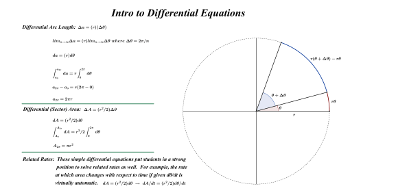
Rates of change (and related rates) can very easily be folded into the fabric of our work from thoughtful consideration of the topic shown above.  This is a necessary outcome as the task of deriving integrals of logarithms, trig functions, etc. is too demanding at this level.  Derivatives of these functions are, however, well within the grasp of high school students. Once these are derived, the inverse nature of integrals and derivatives can be exploited to continue on our little journey.

I realize that this approach isn’t for everyone but it works for me and my students seem to enjoy their work as well.

That is all for now. Thanks for reading.