Archive for the ‘Calculus: An Introduction’ Category

e^(Pi) vs (Pi)^e

Posted: February 28, 2016 in Calculus: An Introduction
Tags: , ,

Is  e^π > π^e  or  is  e^π < π^e ???

This is a continuation of my Euler-pi theme that seems to have consumed me over the past two days. The answer to the question put forth is easy to determine using technology but little to nothing of value is learned through that process. Natural logarithms, functions and derivatives are once again employed here to arrive at a logical (to me) conclusion.
e and pi
e vs pi2


Click on the link provided here for an exploration of the tangent line as it moves along the function.

This entry opens a discussion on “local” versus “global” extrema as well as indeterminate limits.

Click on L’Hospital’s Rule to see the limit of  x/ln(x)  as  x→∞.


Thanks for reading.


For the past several weeks, I’ve been subjected to an advertisement on television (the rule of 72). It then occurred to me that this might be a mystery to many (my students included) who have been witness to the same. This entry is my response to any curiosities that might exist with respect to the “Rule of 72”.

My initial plan was to pick things up where the formula for compound interest left off. I then reconsidered and decided to include a quick derivation of that formula as well.


Compound Interest

Rule of 72

Having the formula for compound interest in place allows us to move forward and uncover the “mystery behind the Rule of 72.


Rule of 72

Rule of 72b

Click on the link provided here to learn about the Euler constant “e”.


Thanks for reading.

Taylor Series

Posted: February 27, 2016 in Calculus: An Introduction
Tags:

Suppose we would like to approximate a function f(x) by some simpler polynomial function g(x) near some value “x=a” (radius of convergence). The result is referred to as the Taylor Series (or Taylor expansion) of the function f(x).

To keep things tidy, the examples here will involve polynomial approximations of f(x) near “x=0”. The constant term (y-intercept) of the original function f(x) and its polynomial approximation are easily determined; it would simply be “f(0)”. It stands to reason that the slopes of the functions in question must be equal to one another at “x=0″ as well. Hence, f'(0) must therefore equal to g'(0). The same argument holds true for the second, third, fourth derivatives and so on. Our goal is to represent the parameters of g(x) in terms of f(0), f'(0), f”(0), etc.

The result of the process outlined above is called the “Taylor Series”. The template for this series will be fleshed out below and then applied to several well-known functions to arrive at their polynomial approximations.


Taylor Series Derived

Taylor Series Derived

Applying any new concept and comparing with what is already known is always good practice. Below, the Taylor expansion is applied to three functions that are very familiar to high school students. The links that follow provide students the opportunity to interact and explore how the Taylor Series behaves as  “n”  increases without bound.


e^x, sin(x) and cos(x)

Taylor Expansion e^x sin(x) cos(x)

Click on the following links to explore each function.

f(x)=e^x , f(x)=sin(x) ,  f(x)=cos(x)

Having seen the Taylor expansion for the three functions above, the stage is now set up very nicely to bring this entry to its conclusion.


Euler’s Formula

Euler's Formula

Thanks for reading.


Reference

Courant, Richard., John, Fritz (1999).  Introduction to Calculus and Analytics:                                     Classics of Mathematics. New York, NY:  Springer-Verlag Berlin Heidelberg.

Euler: The Intro Continues

Posted: February 27, 2016 in Calculus: An Introduction
Tags:

There are many great explorations to pursue in Math 31 (introduction to Calculus) of which we owe thanks to Leibniz, Newton and many others who followed. With “π” week fast approaching, it is an appropriate time to further introduce my students to the genius of Swiss mathematician Leonhard Euler.

This entry begins with a step function that appears to converge on π. Through our little journey here, students will understand and develop the reasoning used by Euler to show that the infinite series 1/n^2 does in fact converge.

Euler pi

What’s going on here and why is this thing approaching π???


To have any chance of understanding this, we need to build on what students already know. The following set-up is crucial.

(pi)squaredBY6

The notes directly above are well within the abilities of high school students to conceptualize; these same concepts and procedures will now be transferred to a new context that students are not so familiar with. The Taylor Series allows us to approximate many functions very accurately (within the vicinity of some value of “x”) as polynomial functions. The polynomial representation of f(x)=sin(x) will be exploited here to arrive at our destination.


Taylor Series

(pi)squaredBY6(b)

sin(x)


Students are well-versed in expressing polynomial functions in factored form as shown below; an appropriate comparison is eventually made to end our little journey.

(pi)squaredBY6(c)

Thanks for reading.


Reference

Courant, Richard., John, Fritz (1999).  Introduction to Calculus and Analytics: Classics of Mathematics. New York, NY:  Springer-Verlag Berlin Heidelberg.

In accordance with normal procedures, previously addressed topics are once again reflected on in this entry. Directly below, the derivative of e^x is dealt with from the perspectives of slope fields and differential equations. Beneath that, the derivative of e^x is considered as a Taylor Series.

Slope Field

Taylor Series Diff Equations2


Taylor Series

Taylor Series Diff Equations2Taylor

It is easy for high school students to determine that dy/dx = y for the Taylor Series representation of e^x above. This sets the stage very nicely for an exploration into power series which, in turn, lead directly to some other very cool “discoveries”. Follow the link provided for a more conventional extraction of the derivative of e^x.

Thanks for reading.


Reference

Courant, Richard., John, Fritz (1999).  Introduction to Calculus and Analytics: Classics of Mathematics. New York, NY:  Springer-Verlag Berlin Heidelberg.

As in the case of the cone, volume of the pyramid can be determined in various ways. The version here once again dabbles with a multi-variable scenario to give students some variation on a familiar theme.

Pyramid Volume2

Click on the link to interact with the notion of infinitesimals as applied to pyramid volume.

Refer to volume of cone for helpful comparison.


Thanks for reading.

The Least Squares Method is based upon the square of the vertical distance (error) from each point given to a general function; this function can be linear, quadratic, cubic, etc. in nature.

Squaring the errors mentioned above alleviates the “+/-” issue that arises from the fact that some points are above and others below the desired function. The sum of these “errors^2” (E) must then be differentiated with respect to each of the parameters found in the general function being used.

There will be two partial derivatives for linear functions, three for quadratic functions, and so. Each partial derivative is then set equal to zero, since our objective is to minimize the error. For linear regression, the result will produce two equations, each in two variables; quadratic regression yields three equations in three variables, etc., etc., etc…… These equations must be solved in such a way as to find values of all parameters that meet, simultaneously, the objectives set forth (minimizing the error).

Students will recognize very quickly from their work in Math 20-1 the systems of equations in two variables that emerge from the linear regression shown below. By exploiting matrix operations on their graphing calculators, students can make quick work of solving simultaneous equations in three (or more) variables. This would be a perfect spot from which to launch the study of linear combinations of vectors; a completely different perspective on minimizing errors awaits here.

Partial Derivatives:  When differentiating with respect to a particular parameter, all other parameters are considered as constants.


Linear Regression

Least Squares

Click on the link provided to explore linear regression.


In the spirit of consistency, I’ve included a quadratic regression below for comparison to the previous linear counterpart.

Quadratic Regression

Least SquaresQuadratic

Click on the link provided to explore quadratic regression.


As mentioned earlier, the subject of this entry provides a very nice point from which to commence the study of linear combinations; that perspective will eventually be linked here.


Thanks for reading.

Now that the formula for arc length has been determined, we can pursue surface areas of curved solids.

Some students have great difficulty conceptualizing areas on curved surfaces. The problem lies in the fact that they want to use Δx or Δy in the setup, just as they did when calculating volumes of solids and areas over flat surfaces. Since on a curved surface, both x and y are changing in unison; as one changes, so does the other. For this reason, we need to use a variable linking those two variables together. This brings into play the Pythagorean Theorem and arc length. Arc length is a one-dimensional measure, its formula the result of capturing the interplay between Δx and Δy and expressing that as Δs. Integrating the one-dimensional Δs over a given interval will therefore produce the desired outcome (even though the path might not be linear, its distance is nevertheless one-dimensional).

A similar argument can be made for calculating areas over curved surfaces. Since area is two-dimensional, the integral we set up to calculate area must stick to that. I visualize a sphere wrapped with very narrow “bands”. If one of these bands was removed and cut, it could be stretched out and laid flat; its length on one edge would exceed that of the opposing edge due to the fact that it was wrapped around a curved surface. Ultimately this is not a problem, however, since these two opposing edges approach the same length as the distance between them narrows. This is entirely similar to each annulus in a previous post where circle area was derived using the “onion proof“.

This takes care of one dimension required for surface area. The second dimension is arc length mentioned in paragraph two above. As  Δs approaches zero, the line segment joining the two infinitely close points that determine the “point” of tangency becomes ever more perpendicular to the length of each band mentioned earlier. Each band can be treated as a rectangle; area is determined as the product of width (arc length) and length (circumference of 3-D solid) at each x_i over the given interval.


The following notes reveal surface area of a sphere using the reasoning described above.

Sphere

Surface Area (sphere)Conventional

Click on the link to view the changing width of each “band” around the sphere.


As before, students can once again benefit having a second example from which to draw comparisons to the first; the cone serves this purpose very well.

Lateral Surface Area of Cone

Cone Lateral Area


Thanks for reading.

Surface areas of curved 3-dimensional solids tend to be much more difficult for students to conceptualize than those whose sides do not stray from a “level” plane. These will eventually be addressed but we will first discover how to calculate lengths of curves.

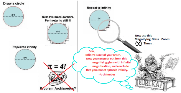
The circle will once again be called upon to initiate this exploration; the image below illustrates, in part, the method of exhaustion that Archimedes utilized to arrive at his estimate for π.

Archimedes Circumference2

Click on the link here to interact with what Archimedes revealed.


……..and now this. Was Archimedes wrong???

IMG_5215

Source: math.stackexchange.com

If the fellow above had joined pairs of points at each successive corner with a line segment (hypotenuse) and based his calculation for circumference on the sum of those, he would have found that Archimedes was correct all along.
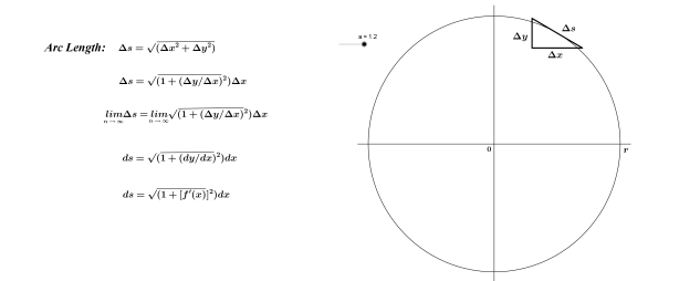
 

Arc Length Formula

As  Δs approaches zero in this exploration, its length becomes a more accurate estimate for the arc length near the “point” of tangency (there are always two points in very close proximity). The end result through the limiting process shown directly below is the formula for arc length.

ArcLength Circle

Its always beneficial for students to work through several examples to cement their understanding of new concepts and related procedures; my preference is to provide examples that are already familiar to them. Calculating arc length (in this case) can then serve as a verification and acceptance of the new concept is achieved with confidence. The offering directly below and the link that follows connects the arc length formula to the Pythagorean theorem.

Arc Length

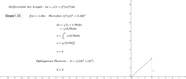
The formula for arc length is based on the Pythagorean theorem; it is therefore not surprising that they produce the same lengths on linear functions.


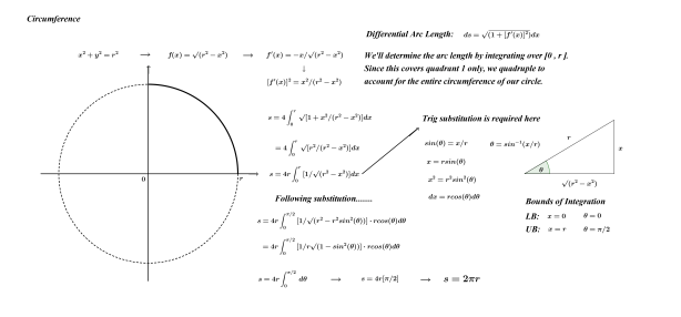
The real power of the formula for arc length lies in its applications to curves. Since students have known the circle’s circumference for several years, it is appropriate to now derive 2πr using our new tool. This is shown below and once again brings trigonometric substitution into play.

Circumference of the Circle

Arc Length (Circumference of Circle)

Once the circle’s circumference has been established using the arc length formula, the integration process can be further solidified by using arc length to once again calculate the circle’s area.


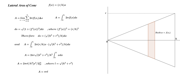
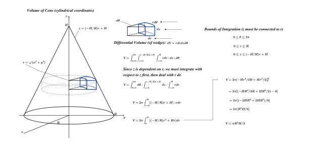
The formula for arc length will once again be employed in deriving the formulas for surface area of the sphere and cone.


Thanks for reading.


This entry will no doubt get further under the skin of those who contend that I’m pushing things too far (and that is exactly why I’m publishing it).  This is a natural extension of the 2-dimensional analog in which circle area was derived. Cylindrical coordinates are identical to polar coordinates with a 3rd dimension thrown in. Directly below, the vertical dimension is governed by a linear function which results in a cone.

In the spirit of consistency, I’ve included a second example with which to draw comparisons to the first. Everything is identical between the two cases with one exception; the function which governs the vertical dimension in example two is that of a semi-circle.


Volume of a Cone

VolumeCone Cylindrical

Interact with cylindrical coordinates to see how the 3-dimensional sector changes.


Volume of a Sphere

VolumeSphere Cylindrical


Thanks for reading.